3D cephalometric landmark detection by multiple stage deep reinforcement learning

Subjects and CT data

CT data from our previous 3D cephalometric study of normal subjects were used²⁶. Twenty-eight normal Korean adults with skeletal class I occlusion volunteered, informed consent being obtained from each subject. The work was approved by the Local Ethics Committee of the Dental College Hospital, Yonsei University, Seoul, Korea (IRB number: 2-2009-0026). All methods were carried out in accordance with relevant guidelines and regulations in the manuscript. Both clinical and radiographic examinations were used to rule out facial dysmorphosis, malocclusion, or history of surgical or dental treatment. The subjects were anonymized and divided into two groups, the training group (n = 20) and the test group (n = 8).

Landmarks

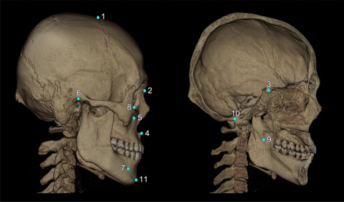
The following craniofacial and mandibular cephalometric landmarks (total N = 16) were included in this study (Fig. 3): bregma, nasion, center of foramen magnum, sella turcica, anterior nasal spine, pogonion, orbitale, porion, infraorbital foramen, mandibular foramen, and mental foramen. The latter five points were bilateral, and the others unilateral. These points are applicable to general cephalometric analysis, but may not be sufficient for a specific analysis, such as Delaire’s²⁶. Each landmark’s definition, position, and type is described in Fig. 3 and Supplementary Table 1.

3D cephalometric landmarks used in this study were marked on the skull, some of them on the surface and others inside the skull; others were in the confined space. The total number of landmarks was 16, five being bilateral. All landmarks are defined and explained in Supplementary Table 1. They are also classified into three landmark types according to Bookstein’s landmark classification, as seen below in notes 2–4. Note (1) the name of landmarks used in this study: 1. bregma; 2. nasion; 3. sella; 4. anterior nasal spine (ANS); 5. infraorbital foramen (IOF, bilateral); 6. porion (bilateral); 7. mental foramen (MF, bilateral); 8. orbitale (bilateral); 9. mandibular foramen (F, bilateral); 10. center of foramen magnum (CFM); 11. Pogonion. Note (2) Type 1 landmarks (n = 2): bregma, nasion. Note (3) Type 2 landmarks (n = 8): sella, anterior nasal spine, infraorbital foramen, orbitale, mental foramen. Note (4) Type 3 landmarks (n = 6); porion, center of foramen magnum, mandibular foramen, pogonion.

Two experts, each having done 3D cephalometry for more than 10 years in a university hospital setting, independently located these 16 landmarks for 3D cephalometric analysis with Simplant software (Materialise Dental, Leuven, Belgium)²⁷. Their mean landmark coordinate values were used as the standard to evaluate DRL prediction accuracy in this study. The coordinate value on the (x)-axis indicated the transverse dimension, the (y)-axis the anterior–posterior dimension and the (z)-axis the top–bottom dimension. The coordinate value of each landmark in Simplant software was exported in Digital Imaging and Communications in Medicine (DICOM) format to construct the label data using the StoA software (Korea Copyright Commission No. C-2019-032537; National Institute for Mathematical Sciences, Daejeon, Korea).

The landmarks have different characteristics which can be classified into three types based on their structural location and informed by biological processes and epigenetic factors^28,29. Although landmark typing is not highly consistent across several studies²⁹, we classified them into three types^28,29, as follows: the type 1 landmark (on discrete juxtaposition of tissues), including bregma and nasion; the type 2 point (on maxima of curvature or local morphogenetic processes), involving sella, anterior nasal spine, infraorbital foramen, orbitale, and mental foramen; finally, type 3 points, comprising porion, center of foramen magnum, mandibular foramen, and pogonion.

General scheme

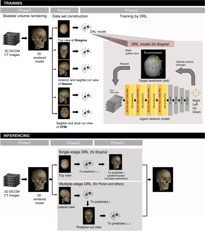
CT data in DICOM format were transferred to a personal computer and a volume rendered 3D model was produced by the following steps: a 2D-projection image was acquired by ray-casting, and the transparency transfer function was applied for bone setting (as shown in the first phase of training in Fig. 4). To compose the dataset, we adjusted the image for each landmark by anatomical view in gray and to (512times 512) in pixel size. The adopted main views were top, bottom, anterior, posterior, or lateral (right or left) view of the 3D model and their cutaway views (defined as a 3D graphic view or drawing in which surface elements of the 3D model are selectively removed to make internal features visible without sacrificing the outer context entirely), as shown in Fig. 1C,E,F. To locate the landmark on cutaway view, voxel pre-processing was performed with transparency application in the region of no interest. A dataset was constructed by combining the obtained images and labelled landmark with its pixel location in the corresponding image view domain, which had been converted from DICOM coordinates to image pixel coordinate.

Schematic diagram of the proposed 3D cephalometric landmark detection framework using deep reinforcement learning (DRL). The training stage included data import and volume rendering in the first phase, anatomical image view adjustment for landmarks in the second phase, and training with DRL agents in the third phase. The latter is depicted in detail in the upper box with a drawing to illustrate the agent navigating toward the target landmark. The inferencing stage included both single- and multi-stage DRL, starting with the same 3D model rendering in phase 1, followed by single-stage or multi-stage DRL in the second phase, and finalized by gradient-based boundary estimation for single-stage DRL, or by repeated DRL and landmark prediction for multi-stage DRL in the third phase.

Single or multiple views were appropriately produced for each landmark and DRL training was performed without data augmentation on the 20 training group models (as shown in the second and third phases of the training stage in Fig. 4). DRL training was organized in such a way that the environment responds to the agent’s action and the agent continuously acts to get maximum rewards from the environment¹⁷, i.e., to reach the closest location to the reference coordinate (as shown in the third phase of training in Fig. 4).

At the inferencing stage, landmark prediction was performed by both single-stage and multi-stage DRL to evaluate the landmark- or stage-related accuracy level (as shown in the first phase of inference stage in Fig. 4). Single-stage DRL refers to one pass of the DRL algorithm, followed by gradient-based boundary estimation, for landmark detection. The multi-stage DRL was defined as the application of a single-stage DRL algorithm for more than two passes, without the gradient-based boundary estimation. The single-stage DRL was not applicable to landmarks located in 3D empty space, such as foramen magnum or sella. These landmarks therefore needed to be determined by multi-stage DRL, whereas other points could be inferenced by both single- and multi-stage DRL (as shown in the second and third phase of the inferencing stage in Fig. 4).

DRL for cephalometric landmark detection

The DRL training framework known as Double DQN³⁰ was adopted after comparing its performance with that of other DQNs for 3D landmarking. DQN handles unstable learning and sequential sample correlation by applying the experience replay buffer and the target network, achieving human-level performance³¹. Double DQN achieves more stable learning by utilizing the DQN solution to the bias problem of maximum expected value³⁰.

The DRL agent learns the optimal path trajectory to a labeled target position through a sequential decision process. We formulated the cephalometric landmark detection problem as a Markov decision process, defined by (mathcal{M}=(mathcal{S},mathcal{A},mathcal{P},mathcal{R})) where (mathcal{S}) is the set of states, (mathcal{A}) set of actions, (mathcal{P}) the state transition probabilities, and (mathcal{R}) the reward function. In this study, environment (E) is an image ((512times 512)) obtained through volume rendering from DICOM data with ground truth landmark position. The agent’s action (ain mathcal{A}) was defined as movements on the 2D image plane (right, left, up, and down), along the orthogonal axis in an environment image. The state (sin mathcal{S}) was defined as a region of interest image from the environment wherein the agent was located. It was zoomed to various pixel resolutions with a fixed pixel size of (128times 128). The reward function ({mathcal{R}}_{t}) was defined by the Euclidean distance between the previous and current agents at time (t) as follows:

where (AP) represents the predicted image position on the image of given (E), and (TP) is the target ground truth position. The agent receives a reward from the environment after valid action in every step. The state action function (Q(s,a)) is then defined as the expectation of cumulative reward in the future with discount factor (gamma). More precisely,

Using the Bellman optimality equation³², the optimal state action function ({Q}^{*}(s,a)) for obtaining the optimal action is computed as the following:

Q-learning finds the optimal action-selection policy by solving Eq. (3) iteratively³³. Due to the heavy computation needed, an approximation by the deep neural network (Qleft(s,a;theta right)) was adopted instead of (Qleft(s,aright)), where (theta) is the parameter of the deep neural network. Double DQN algorithm minimizes the function (L(theta )) as defined by the following:

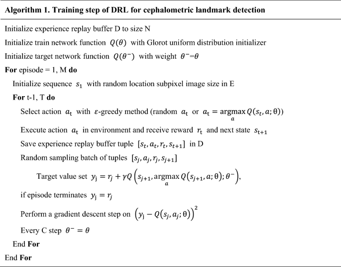
where ({theta }^{-}) represents the frozen target network parameters. The target network ({Q(theta }^{-})) was periodically updated by parameter values copied from the training network (Qleft(theta right)) at every (C) step. The update frequency (C) of the target network was empirically set to check the convergence of the loss function. Gradient clipping was applied to limit the value within ([-1, 1]), as suggested by Mnih et al.³¹. To avoid the sequential sample correlation problem, experience replay buffers (denoted by (D)) were used, consisting of multi-scale resolution patch images ((128times 128)) extracted by the agent’s action in our training process. Random sampling tuples ([{s}_{t}, {a}_{t}, {r}_{t}, {s}_{t+1}]) were configured in batches and trained³¹. Details of training steps for our DRL are described in Algorithm 1 (in pseudocode) and Fig. 4. A multi-scale agent strategy was used in a coarse-to-fine resolution manner^23,24,25. Our termination condition was set to the case of fine resolution and the most duplicate agent position in the inferencing phase.

The agent network contained four convolutional layers with (128times 128times 4) as input (frame history (k) is 4), each followed by a leaky rectified linear unit, and four (2times 2) max pooling with stride 2 for down-sampling. The first and second convolutional layers convolved 32 filters of (5times5). The third and fourth convolutional layers convolved 64 filters of (3times 3). All convolutional layers’ stride was 1. The last pooling layer was followed by four fully-connected layers and consisted of 512, 256, 128, and 4 rectifier units, respectively. The final fully-connected layer had four outputs with linear activation. All layer parameters were initialized according to the Glorot uniform distribution. Figure 4 illustrates the agent network model in the third phase of the training stage.

Single-stage DRL

As single-stage DRL is simpler than the multi-stage approach, only two components of 3D coordinates for a landmark could be obtained. The remaining one-dimensional coordinate was inferred by a gradient-based boundary estimation (as shown in the second and third phases of the inferencing stage in Figs. 4 and 5).

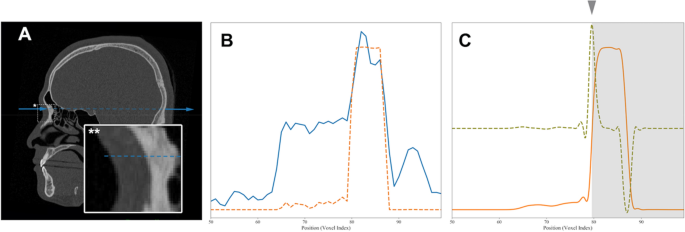
Gradient-based boundary estimation for single-stage DRL. (A) A sectional CT image in the sagittal plane with a radiographic beam-mimic line (blue dashed line) passing through a sampled landmark, nasion and surrounding box with asterisk (*). The view of the box region is magnified in the inset box at the left bottom with double asterisks (**) and the y-directional line (blue solid). (B) One-dimensional plot of image density profile in Hounsfield units, shown as a blue solid line along the y-directional line passing through the air, through nasion, and the soft and bone tissue, indicated by the blue dashed line in Fig. A. The orange dashed line indicates the bone intensity-enhanced profile. (C) Plot of the same source for B showing the non-linear diffusion profile of the bone intensity-enhanced one (orange solid line), its first order derivative profile (light green dashed line), and the final boundary estimation of bone (marked by arrowhead and gray region).

The obtained steep gradient changes in CT values at the boundary between the soft tissue and cortical bone (as seen in Fig. 5A) were used to detect the depth of the landmark. If we want to get a landmark on the surface of bone, for example, the nasion point, we first get (x) and (z) values of the 3D coordinate by applying the single-stage DRL algorithm on the anterior view of skull. The remaining one-dimensional profile of CT value along the (y)-axis at point (x) and (z) can then be obtained by robust boundary detection using the gradient values that we propose here, the bone intensity enhancing function (IE(x)) being defined as follows:

where (x) is the CT value, (L) is the center of the CT value range, and (W) is a scale value. (L) was 400 and (W) was 200 for our study. The application of (IE(x)) turns a one-dimensional profile of CT value (blue line in Fig. 5A) into a simple profile with enhanced bone intensity (orange line of Fig. 5B). The robust calculation of the gradient, however, may suffer from noise contamination. We therefore apply a non-linear diffusion equation using the structure tensor to remove the noise without losing the gradient information³⁴. After taking the first order derivative of the noise-reduced profile, the location with maximal gradient is set to the detected bone surface position to determine the remaining coordinate value. Please see Fig. 5C for more details.

Multi-stage DRL

During our application of multi-stage DRL, the first DRL procedure predicted two coordinate values of a landmark, and these values were used to make the predicted axis for constructing a cutting plane and a new cutaway view. A second DRL was then performed on the newly-constructed cutaway view to calculate the coordinate values again. Most of the landmarks in this study were predicted with excellent accuracy by the first and second DRL, i.e., two-stage DRL, but some landmarks, such as infraorbital foramen, did not yield a satisfactory level of accuracy until the third stage.

Figure 1A–C show sample views of multi-stage DRL with various 3D and cutaway views to determine the right side orbitale point (marked as a light blue point). The (x) and (z) coordinate value of right orbitale was predicted by the first DRL on the anterior view of the 3D skull, as shown in Fig. 1A. The sagittal-cut left lateral view was produced for the remaining coordinate value based on the previously determined (x) coordinate value (Fig. 1B,C); (y) and (mathrm{z}) values were then finally determined by the second DRL agent, as in Fig. 1C.

The prediction of a landmark located inside the skull, such as sella point, was also achieved: two coordinate values of (y) and (z) were initially predicted by the first DRL on the median-cutaway left half skull (Fig. 1D,E). This was followed by the construction of another cutaway, based on the previous (mathrm{z}) coordinate value, to produce an axial-cut top view (Fig. 1F). Finally, the second DRL could predict (x) and (y) coordinate values, as presented in Fig. 1F.

Implementation

The visualization toolkit was used for the 3D volume rendering³⁵. Double DQN implementation is based on the open source framework for landmark detection²⁵. The computing environment included Intel Core i9-7900X CPU, 128 GB memory, and Nvidia Titan Xp GPU (12 GB). We set the batch size to 96, discount factor (gamma) to 0.9, and experience replay memory size to ({10}^{6}). We also applied adadelta, an adaptive gradient method for an optimizer. It took approximately 90–120 h to train each individual landmark training model, while inferencing took 0.2 s on average for the landmark detection of a single image view.