Deep learning model for analyzing the relationship between mandibular third molar and inferior alveolar nerve in panoramic radiography

Study design

This study analyzed the diagnostic performance of the positional relationship between the inferior alveolar canal/nerve and the mandibular third molar from panoramic radiographs using an optimized CNN deep learning model.

Ethics statement

This study was approved by the Institutional Review Board of Kagawa Prefectural Central Hospital (approval number: 1023; approval date: 8th March 2021). The board reviewed our retrospective non-interventional study design and analytical study with anonymized data and waived written documentation of personal informed consent. All methods were performed following the relevant guidelines and regulations. The study was registered at jRCT (jRCT1060220021).

Preparation of image datasets

We retrospectively used radiographic imaging data collected at the Department of Oral and Maxillofacial Surgery in a single general hospital from April 2014 to December 2021. The study data included patients aged 20–76 years in the mature mandibular third molar who had panoramic radiographs and CT taken on the same day. This study confirms the positional relationship between the mandibular third molar and the inferior alveolar canals by panoramic radiography. An unclear image (three teeth) and an image of the remaining titanium plate after the mandibular fracture (one tooth) were excluded. Finally, 1279 tooth images were used in this study.

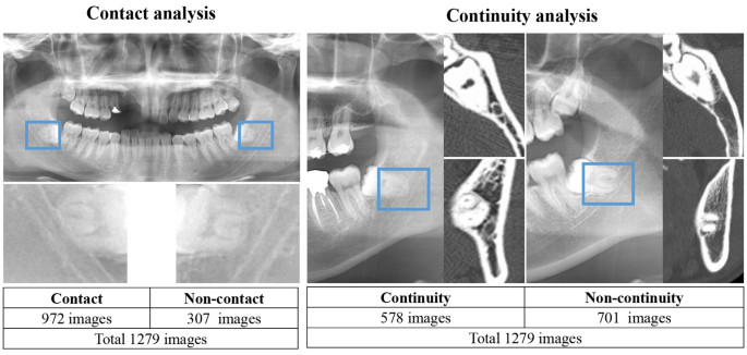
Digital image data were obtained using dental panoramic radiographs taken with either of the two imaging devices (AZ3000CMR or Hyper-G CMF; ASAHIRENTOGEN Ind. Co., Ltd., Kyoto, Japan). All digital image data were output in a tagged image file format (digital image size: 2776 × 1450, 2804 × 1450, 2694 × 1450, or 2964 × 1464 pixels) using the Kagawa Prefectural Central Hospital Picture Archiving and Communication Systems system (Hope Dr. Able-GX, Fujitsu Co., Tokyo, Japan). Under the supervision of an expert oral and maxillofacial surgeon, two oral and maxillofacial surgeons used Photoshop Elements (Adobe Systems, Inc., San Jose, CA, USA) to crop the areas of interest manually. The image was cropped by selecting the area, including the apex of the mandibular third molar and the inferior alveolar canal within 250 × 200 pixels (Fig. 1). Each cropped image had a resolution of 96 dpi and was saved in the portable network graphic format.

Classification of the relationship between the mandibular third molar and inferior alveolar canal/nerve.

Classification of mandibular third molar and inferior alveolar nerve

First, using panoramic radiographs, we classified the contact and superimposition between the mandibular third molar and inferior alveolar canal. This is because contact between the inferior alveolar duct on panoramic radiographs is a risk factor for nerve exposure^4,20.

Second, we classified the presence or absence of direct contact between the mandibular third molar and inferior alveolar nerve using CT. The classification criteria and distributions are as follows and are also shown in Fig. 1.

1. 1.

   Relationship between the mandibular third molar and inferior alveolar canal.

   1. (a)

      Non-contact or superimposition of the mandibular third molar and inferior alveolar canal.

   2. (b)

      Contact or superimposition between the mandibular third molar and the inferior alveolar canal.

In this study, contacts and superimposition/overlaps were grouped together.

1. 2.

   Relationship between the mandibular third molar and inferior alveolar nerve.

If there was discontinuity of the cortical bone at the inferior alveolar canal due to the mandibular third molar, it was classified as a defect.

1. (a)

   Contact between the mandibular third molar and inferior alveolar nerve (i.e., defect or discontinuity in the cortical bone of the inferior alveolar canal).

2. (b)

   Non-contact between the mandibular third molar and inferior alveolar nerve (i.e., continuity of the cortical bone of the inferior alveolar canal).

CNN model architecture

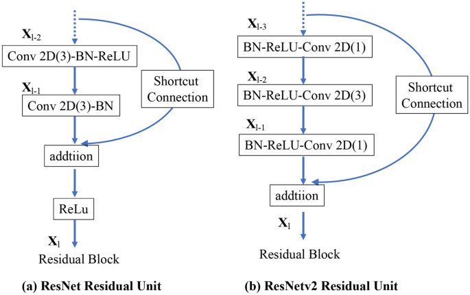
ResNet50 is a 50-layer deep CNN model. Traditional CNNs have the major drawback of the “vanishing gradient problem,” where the gradient value is significantly reduced during backpropagation, resulting in little weight change. The ResNet CNN model uses a residual module to overcome this problem²¹. ResNet v2 is an improved version of the original ResNet²², with the following improvements compared with the original ResNet (Fig. 2): (1) The shortcut path is completely identity mapped without using the ReLU between the input and output. (2) After branching for the residual calculation, the order is changed to batch normalization²³ as -ReLU-convolution-batch normalization-convolution.

Differences between the residual blocks of ResNet and ResNetv2: (a) ResNet Residual Unit; (b) ResNetv2 Residual Unit. BN: Batch Normalization and Conv2D: Two-dimensional convolution layer.

In this study, we selected two CNN models, ResNet50 and ResNet50v2. The ResNet50 and ResNet50v2 CNN models were pre-trained on the ImageNet database and fine-tuned according to the positional relationship classification task for the mandibular third molar and inferior alveolar nerve. The deep learning task process was implemented using Python (version 3.7.13), Keras (version 2.8.0), and TensorFlow (version 2.8.0).

Dataset and CNN model training

Each CNN model training was generalized using K-fold cross-validation in the deep learning algorithm. The models were validated using tenfold cross-validation to ensure internal validity. The digital image dataset was divided into ten random subsets using the stratified sampling technique, and the same classification distribution was maintained for training, validation, and testing across all subsets²⁴. The dataset was split into separate test and training datasets in a ratio of 0.1–0.9 within each fold. Additionally, the validation data comprised one-tenth of the training dataset. The model averaged ten training iterations to obtain prediction results for the entire dataset, with each iteration retaining a different subset for validation.

The cross-entropy—defined by Eq. (1)—was used for the loss function.

where t_i is true label and y_i is the predicted probability of class i.

Optimization algorithm

This study used two deep learning gradient methods, stochastic gradient descent (SGD) and sharpness-aware minimization (SAM). SGD is a typical optimization method in which the parameters are updated by the magnitude in the obtained gradient direction. The momentum SDG is a method of adding momentum to SGD²⁵. In this study, the momentum was set to 0.9. The momentum SGD is expressed in Eqs. (2) and (3).

where w_t is t-th parameter, η is learning rate, ∇L (w) is differentiation with parameters of the loss function, and α is momentum.

SAM is an optimization method that converges to a parameter with minimal loss and flat surroundings²⁶. It uses a combination of a base optimizer and SAM to determine the final parameters using traditional algorithms. SGD was selected as the base optimizer. The loss function of SAM is defined by Eq. (4). This is used to minimize Eq. (5).

where S is the set of data, w is a parameter, λ is the L2 regularization coefficient, L_s is the loss function, and ρ is the neighborhood size.

This study analyzed the deep learning models using a ρ value of 0.025.

Deep learning procedure

Data augmentation

Data augmentation prevents excessive adaptation to the training data by diversifying the input data²⁷. The following values were selected for the preprocessing layer to convert the images during training randomly. The boundary surface of the missing part was complemented by folding back using the reflect method.

• Random rotation: range of − 18° to 18°

• Random flip: horizontally and vertically

• Random translation: up–down and left–right range of 30%

Learning rate scheduler

Learning rate decay is a technique used to improve the generalization performance of deep learning and reduce the learning rate from a state in which learning has progressed to some extent. Decay in the learning rate can improve accuracy²¹. The changes due to time-based decay as a learning rate can be found in the appendix. The learning rate decay can be evaluated using Eq. (6).

The learning rate scheduler was executed with an initial learning rate of 0.01 and a decay rate of 0.001. All the models conducted analysis over 300 epochs and with 32 batch sizes without early stopping. These deep learning processes were repeated 30 times for all models using different random seeds for each analysis.

Performance metrics and statistical analysis

To evaluate the performance of each deep learning model, the accuracy, precision, recall, F1 score, and area under the curve (AUC)—calculated from the receiver operating characteristic (ROC) curve—performance metrics were employed. More detailed information on the performance metrics used in this study is present in the Appendix.

Statistical evaluations of the performance for each deep learning model were performed on the data that were independently and repeatedly analyzed 30 times. Data were recorded and stored in an electronic database using Microsoft Excel (Microsoft Inc., Redmond, WA, USA). The database was created and analyzed by using JMP Statistical Software Package Version 14.2.0 for Macintosh (SAS Institute Inc., Cary, NC, USA). All statistical analyses were bilateral with a significance level of 0.05. Normal distribution was evaluated by using the Shapiro–Wilk test. A comparison of classification performance between each CNN model was performed for each metric by using the Wilcoxon signed rank sum test. Effect sizes²⁸ were evaluated using Hedges’ g (unbiased Cohen’s d), Eqs. (7) and (8).

where M1 and M2 are the mean values for the CNN models with SGD and SAM, s1 and s2 are the standard deviations for the CNN models with SGD and SAM, respectively; and n1 and n2 are the numbers for the CNN models with SGD and SAM, respectively. Effect sizes were categorized as large effect, ≥ 2.0; very large effect, 1.0; large effect, 0.8; medium effect, 0.5; small effect, 0.2; and very small effect, 0.01 based on the criteria proposed by Cohen and extended by Sawilowsky²⁹.

Visualization of judgment regions in deep learning

In this study, the gradient-weighted class activation map (Grad-CAM) algorithm³⁰ was used to visualize the noticeable areas of the image in a heatmap. Grad-CAM is a class activation mapping method that uses gradients for weights adopted by the IEEE International Conference on Computer Vision in 2017 and provides a visual basis for deep learning to improve the explanation of the architecture. Grad-CAM uses the last convolution layer of the ResNet model to visualize the feature area.