Evaluation of multi-task learning in deep learning-based positioning classification of mandibular third molars

Study design

The purpose of this study was to evaluate the classification accuracy of CNN-based deep learning models using cropped panoramic radiographs according to the Pell and Gregory, and Winter’s classifications for the location of the mandibular third molars. Supervised learning was chosen as the method for deep learning analysis. We compared the diagnostic accuracy of single-task and multi-task learning.

Data acquisition

We used retrospective radiographic image data collected from April 2014 to December 2020 at a single general hospital. This study was approved by the Institutional Review Boards of the respective institutions hosting this work (the Institutional Review Boards of Kagawa Prefectural Central Hospital, approval number 1020) and was conducted in accordance with the ethical standards of the Declaration of Helsinki and its later amendments. Informed consent was waived for this retrospective study because no protected health information was used by the Institutional Review Boards of Kagawa Prefectural Central Hospital. Study data included patient’s aged 16–76 years who had panoramic radiographs taken at our hospital prior to extracting their mandibular third molars.

In the Pell and Gregory classification, the mandibular second molar was the diagnostic criterion. Therefore, cases of mandibular second molar defects, impacted teeth, and residual roots were excluded from this study. Additionally, we excluded cases of unclear images, residual plates after mandibular fracture, and residual third molar root or tooth extraction interruptions. Overall, we excluded residual third molar roots (39 teeth), mandibular second molar defects or residual teeth (15 teeth), impacted mandibular second molars (12 teeth), tooth extraction interruptions of third molars (9 teeth), unclear images (3 teeth), and residual plates after mandibular fracture (1 tooth). In total, 1,330 mandibular third molars were retained for further deep learning analysis.

Data preprocessing

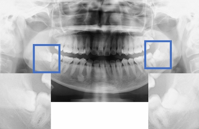
Images were acquired using dental digital panoramic radiographs (AZ3000CMR or Hyper-G CMF, Asahiroentgen Ind. Co., Ltd., Kyoto, Japan). All digital image data were output in Tagged Image File Format format (2964 × 1464, 2694 × 1450, 2776 × 1450, or 2804 × 1450 pixels) via the Kagawa Prefectural Central Hospital Picture Archiving and Communication Systems system (Hope Dr Able-GX, Fujitsu Co., Tokyo, Japan). Two maxillofacial surgeons manually identified areas of interest on the digital panoramic radiographs using Photoshop Elements (Adobe Systems, Inc., San Jose, CA, USA) under the supervision of an expert oral and maxillofacial surgeon. The method of cropping the image was to cut out the mandibular second molar and the ramus of the mandible in the mesio-distal direction and completely include the apex of the mandibular third molar in the vertical direction (Fig. 2). The cropped images had a resolution of 96 dpi/inch, and each cropped image was saved in portable network graphics format.

A depiction of the crop method for data preprocessing.

The manual method of cropping the image involved cutting out the mandibular second molar and the ramus of the mandible in the mesio-distal direction as well as completely including the apex of the mandibular third molar in the vertical direction.

Classification methods

Pell and Gregory classification⁶ is categorized into class and position components. The classification was performed according to the positional relationship between the ramus of the mandible and the mandibular second molar in the mesio-distal direction. The distribution of the mandibular third molar classification is shown in Table 5.

Class I: The distance from the distal surface of the second molar to the anterior margin of the mandibular ramus was larger than the diameter of the third molar crown.

Class II: The distance from the distal surface of the second molar to the anterior margin of the mandibular ramus was smaller than the diameter of the third molar crown.

Class III: Most third molars are present in the ramus of the mandible. Position classification was performed according to the depth of the mandibular second molar.

Level A: The occlusal plane of the third molar was at the same level as the occlusal plane of the second molar.

Level B: The occlusal plane of the third molar is located between the occlusal plane and the cervical margin of the second molar.

Level C: The third molar was below the cervical margin of the second molar.

Based on Winter’s classification, the mandibular third molar is classified into the following six categories^7,14:

Horizontal: The long axis of the third molar is horizontal (from 80° to 100°).

Mesioangular: The third molar is tilted toward the second molar in the mesial direction (from 11° to 79°).

Vertical: The long axis of the third molar is parallel to the long axis of the second molar (from 10° to –10°).

Distoangular: The long axis of the third molar is angled distally and posteriorly away from the second molar (from − 11° to − 79°).

Inverted: The long axis of the third molar is angled distally and posteriorly away from the second molar (from 101° to –80°).

Buccoangular or lingualangular: The impacted tooth is tilted toward the buccal-lingual direction.

CNN model architecture

The study evaluation was performed using the standard deep CNN model (VGG16) proposed by the Oxford University VGG team¹⁵. We performed a normal CNN consisting of a convolutional layer and a pooling layer for a total of 16 layers of weight (i.e., convolutional and fully connected layers).

With efficient model construction, fine-tuning the weight of existing models as initial values for additional learning is possible. Therefore, the VGG 16 model was used to transfer learning with fine-tuning, using pre-trained weights in the ImageNet database¹⁶. The process of deep learning classification was implemented using Python (version 3.7.10) and Keras (version 2.4.3).

Data set and model training

The model training was generalized using K-fold cross-validation in the model training algorithm. Our deep learning models were evaluated using tenfold cross-validation to avoid overfitting and bias and to minimize generalization errors. The dataset was split into ten random subsets using stratified sampling to retain the same class distribution across all subsets. Within each fold, the dataset was split into separate training and test datasets using a 90% to 10% split. The model was trained 10 times to obtain the prediction results for the entire dataset, with each iteration holding a different subset for validation. Data augmentation can be found in the appendix.

Multi-task

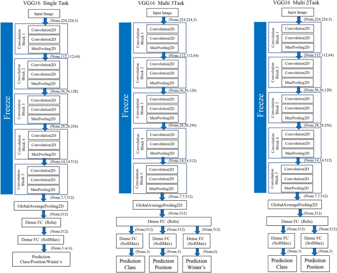
As another approach to the mandibular third molar classifier, a deep neural network with multiple independent outputs was implemented and evaluated. There are two proposed multi-task CNNs. One is a CNN model that can analyze the three tasks of the Pell and Gregory, and Winter’s classifications simultaneously. The other is a CNN model that can simultaneously analyze the class and position classifications that constitute the Pell and Gregory classification. These models can significantly reduce the number of trainable parameters required when using two or three independent CNN models for mandibular third molar classification. The proposed model has a feature learning shared layer that includes a convolutional layer and a max-pooling layer that are shared with two or three separate branches and independent, fully connected layers used for classification. For the classification, two or three separate branches consisting of dense layers were connected to each output layer of the Pell and Gregory, and Winter’s classifications. Each branch included softmax activation. (Fig. 3) Table 6 shows the number of parameters for each of the two types of multi-tasks and single-tasks in the VGG 16 model.

Schematic diagram for classification of the mandibular third molars using single-task and multi-task convolutional neural network (CNN) models.

In the multi-task model, each model was implemented to learn the classification of the mandibular third molars. In both training, the cross entropy calculated in (Eq. 1) was used as the error function. The total error function (L_3total) of the multi-task model for the three proposed tasks is the sum of the Pell and Gregory classification class and position prediction errors (L_cls), (L_pos), and Winter’s classification prediction errors (L_wit) (Eq. 2):

The error function (L_2total) of the entire multi-task model for the two tasks was the total of the prediction errors (L_cls) and (L_pos) of class and position, as well as the Winter’s classification (Eq. 3):

Deep learning procedure

All CNN models were trained and evaluated on a 64-bit Ubuntu 16.04.5 LTS operating system with 8 GB of memory and an NVIDIA GeForce GTX 1080 (8 GB graphics processing unit). The optimizer used stochastic gradient descent with a fixed learning rate of 0.001 and a momentum of 0.9, which achieved the lowest loss on the validation dataset after multiple experiments. The model with the lowest loss in the validation dataset was chosen for inference on the test datasets. Training was performed for 300 epochs with a mini-batch size of 32. The model was trained 10 times in the tenfold cross-validation test, and the result of the entire dataset was obtained as one set. This process was repeated 30 times for each single-task model (for class, position, Winter’s classification), multi-task model (for class and position classification [two tasks], and all three multi-tasks) using different random seeds.

Performance metrics and statistical analysis

We evaluated the performance metrics with precision, recall, and F1 score along with the receiver operating characteristic curve (ROC) and the area under the ROC curve (AUC). The ROC curves were shown for the complete dataset from the tenfold cross-validation, producing the median AUC value. Details on the performance metrics are provided in the Appendix.

The differences between performance metrics were tested using the JMP statistical software package (https://www.jmp.com/ja_jp/home.html, version 14.2.0) for Macintosh (SAS Institute Inc., Cary, NC, USA). Statistical tests were two-sided, and p values < 0.05 were considered statistically significant. Parametric tests were performed based on the results of the Shapiro–Wilk test. For multiple comparisons, Dunnett’s test was performed with single-task as a control.

Differences between each multi-task model and the single-task model were calculated for each performance metric using the Wilcoxon test. Effect sizes were calculated as Hedges’ g (unbiased Cohen’s d) using the following formula¹⁷:

M1 and M2 are the means for the multi-task and single-task models, respectively; s1 and s2 are the standard deviations for the multi-task and single-task models, respectively, and n1 and n2 are the numbers for the multi-task and single-task models, respectively.

The effect size was determined based on the criteria proposed by Cohen et al.¹⁸, such that 0.8 was considered a large effect, 0.5 was considered a moderate effect, and 0.2 was considered a small effect.

Visualization for the CNN model

CNN model visualization helps clarify the most relevant features used for each classification. For added transparency and visualization, this work used the gradient-weighted class activation maps (Grad-CAM) algorithm, which functions by capturing a specific class’s vital features from the last convolutional layer of the CNN model to localize its important areas¹⁹. Image map visualizations are heatmaps of the gradients, with “hotter” colors representing the regions of greater importance for classification.