Identification of osteoporosis using ensemble deep learning model with panoramic radiographs and clinical covariates

Study design

The aim of this study was to classify osteoporosis and non-osteoporosis using a dataset segmented from panoramic radiographs and several different CNNs. Supervised learning was employed as a deep learning method. We statistically investigated the effect of adding covariates extracted from clinical records on the accuracy of the osteoporosis identification.

Data acquisition

We retrospectively used clinical and radiographic data from March 2014 to September 2020. This study protocol was approved by the institutional review boards of the respective institutions hosting this work (i.e., the review boards of Kagawa Prefectural Central Hospital, approval number 994), following Ethical guidelines for clinical research and in accordance with the ethical principles that have their origins in the Declaration of Helsinki and its subsequent amendments. Informed consent from individual patients for this retrospective study was waived at the discretion of the institutional review committee (Kagawa Prefectural Central Hospital Ethics Committee) because protected health information was not used. The study included 902 consecutive images from enrolled patients who underwent panoramic radiography within the first year of receiving DXA at our hospital.

Osteoporosis was diagnosed by the DXA method using the hip or spine. The parameters investigated included the automatically generated BMD (g/cm³) and T-score. Osteoporosis was diagnosed when the T-score of the BMD was less than − 2.5 and non-osteoporosis when the T-score was − 2.5 or more, according to the diagnostic criteria of the World Health Organization²⁹. When DXA was performed at both the hip and spine sites, the result with the lower T-score was used for diagnosis.

The following panoramic radiographs were excluded from this study: 119 images of patients taking antiresorptive agents such as bisphosphonates or anti-RANKL antibodies, 3 images of foreign substances such as plates and gastric tubes, 1 image of a mandibular fracture, and 1 image with poor panoramic radiography. Further analysis was conducted on the remaining 778 images.

Data preprocessing

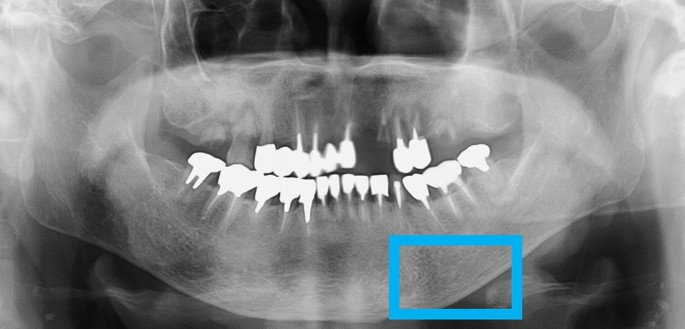
Dental panoramic radiographs of each patient were utilized to acquire images using an AZ3000CMR (ASAHI ROENTGEN IND. Co., Ltd., Kyoto, Japan). All data images were output in .tiff format (2964 × 1464 pixels) from the Kagawa Prefectural Central Hospital PACS system (HOPE DrABLE-GX, FUJITSU Co., Tokyo, Japan). We isolated the cortical bone at the lower edge of the mandible in the images. Two maxillofacial surgeons manually placed and cropped regions of interest (ROIs) on the dental panoramic radiograph images using Photoshop Elements (Adobe Systems, Inc., San Jose, CA, USA). The ROI was set according to previous studies of deep learning that identified the ROI in osteoporosis by panoramic radiography. A previous study identified the middle area of the mandibular lower border as the ROI¹⁷. To ensure reproducibility, the mental foramen was used as the reference point at the mid-point of the mandible. The ROI was created to be 250 × 400 pixels in size just below the reference point to include the lower edge of the mandible. All analyses in this study were performed on the left side, as shown in Fig. 2. The cropped image was saved in PNG format. The oral and maxillofacial surgeons who cropped the image data were completely unaware of the osteoporotic status of each patient as this information was concealed from them according to the experimental design.

Dental panoramic radiographs before deep learning analysis, showing cropped ROI.

CNN model architecture

In this study, the evaluation was performed using the standard CNN models, including a residual neural network (ResNet)¹⁹ and EfficientNet²⁰. ResNet, invented by He et al.¹⁹, won the classification task of the ILSVRC2015 Challenge. Generally, deepening the network layer improves the accuracy of image identification, but conversely, a network layer that is too deep reduces the accuracy. To deal with this issue, we introduced a learning method called residual learning that involves a network that can be deepened to 152 layers. This representative of the ResNet architecture has 18, 50, and 152 layers.

EfficientNet is a CNN that was proposed as a state-of-the-art image classification method on ImageNet data in 2019. Although the number of parameters is smaller than that of the conventional CNN model, EfficientNet is a high-speed and relatively accurate CNN model that uses EfficientNet-b0, -b3, and 0b7 models. For efficient model building³⁰, it is possible to fine-tune the weights of existing models as initial values for additional learning; therefore, all CNNs were used to transfer learning with fine-tuned pre-trained weights using the ImageNet database³¹. The process of deep learning analysis was implemented using the PyTorch deep learning framework and the Python programming language.

Clinical covariates

Patients in the high risk group for osteoporosis are generally female, older, and with lower body mass indices (BMIs)³². There are many other patient factors, but age, gender, and BMI were selected as factors that can be easily identified by dentists. BMI is given by weight in kilograms divided by the square of height in meters. Patients’ weight and height were recorded at the time of BMD measurement. Table 3 shows the clinical and demographic characteristics of the patients in this study.

Architecture of the ensemble model

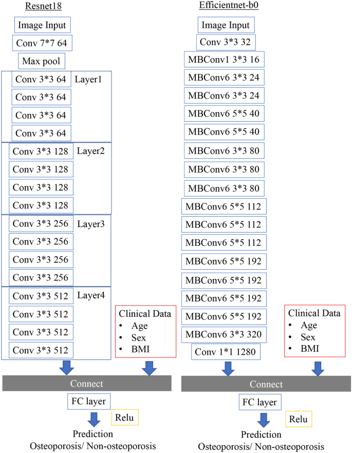
We also constructed an ensemble model that adds patient clinical factors to the deep learning analysis of X-ray images. In preparation, we preprocessed the structural data. Age and BMI were translated into mean normalization, and sex was translated into a one-hot vector representation. As a result, a 1 × 4 dimensional vector was created. Extracted from the convolutional layers in the CNN of the image, the one-dimensional reshaped result and the 1 × 4 dimensional data created from the structural data were combined. The image data processed by CNN and the combined data with clinical covariates were then passed as fully connected layers. The predictions of the final osteoporosis identification model were output using the rectified linear unit (ReLU) activation function (Fig. 3).

Neural network architecture that ensembles image data and clinical covariates. As representative models, ResNet18 and EfficientNet-B0 models are shown.

Data augmentation

Various data augmentation techniques have been used to prevent overfitting owing to the small dataset size. During learning, data augmentation was applied only to the training image data when the images removed in batches. The training images were randomly rotated from − 25 to + 25, with a 50% chance to flip vertically and 50% chance to flip horizontally. The darkness was randomly changed from − 5 to + 5%, and the contrast was changed from − 5 to + 5%. Each training image was processed with a 50% chance of data augmentation.

Model training

The model training was generalized using k-fold cross-validation. The images selected as the dataset were split using the stratified k-fold approach, which splits the training data, validation data, and testing data while maintaining the correct label percentages. The training algorithm used k = 5 for k-fold cross-validation to avoid overfitting and bias and to minimize generalization errors. The data were divided into five sets, and the testing data consisted of 156 images. In each fold, the data set was split into a separate training and validation sets at a ratio of 8:1. The selected validation data set was independent from the training set and was used to evaluate the training status. After completing one model training step, we performed similar validations five times with different testing data.

Deep learning procedure

All deep learning models were trained and analyzed by using the 64-bit Ubuntu 16.04.5 LTS operating system on a workstation with 8 GB memory and an NVIDIA GeForce GTX 1080 8 GB graphics processing unit. The optimizer, weight decay, and momentum were common among all the CNNs. In this study, the optimizer used stochastic gradient descent, with a weight decay of 0 and momentum of 0.9. Learning rates of 0.001 and 0.01 were used for both ResNet and EfficientNet. All the models analyzed a maximum of 100 epochs. We used the early stopping method to terminate the data training to prevent overfitting if the validation error did not update 20 times in a row. This process was performed 30 times on all CNN models for statistical evaluation.

Performance metrics and statistical analysis

Our key performance indicators, namely, the osteoporosis discrimination accuracy, precision, recall, specificity and F1 score, are defined by Eqs. (1), (2), (3), (4), and (5), respectively, which account for the relations between the positive labels of the data and those given by the classifier. We also calculated the ROC curve and measured the AUC.

here TP and TN represent the numbers of true positive and true negative results, respectively, and FP and FN represent the numbers of false positives and false negatives, respectively.

M₁ and M₂ are the means for the ensemble and image-only models; s₁ and s₂, respectively, are the standard deviations for the ensemble and image-only models; and n₁ and n₂, respectively, are the numbers for the ensemble and image-only models.

Statistical analyses were performed for each performance metric with the use of JMP Statistics Software Package Version 14.2.0 for Macintosh (SAS Institute Inc., Cary, NC, USA). P < 0.05 was considered statistically significant, and 95% confidence intervals were calculated. Parametric tests were performed based on the results of the Shapiro–Wilk test. The effect sizes were calculated as Hedges’ g (unbiased Cohen’s d). The effect size was determined as follows based on the criteria proposed by Cohen and expanded by Sawilowsky³³: a very small effect was 0.01, small effect was 0.2, medium effect was 0.5, large effect was 0.8, very large effect was 1.0, and huge effect was 2.0.

Visualization of the computer-assisted diagnostic system

Gradient-weighted class activation mapping (Grad-CAM) is a technology that visualizes important pixels by weighting the gradient with respect to the predicted value³⁴. It shows information that is significant for identification: the high gradient of the input to the last convolutional layer. Guided Grad-CAM is a combination of Grad-CAM and backpropagation visualization techniques that are useful for identifying detailed feature locations. The feature area visualization was reconstructed from the last convolution layer of each CNN in this study.