Protocol for 3D colour reproduction
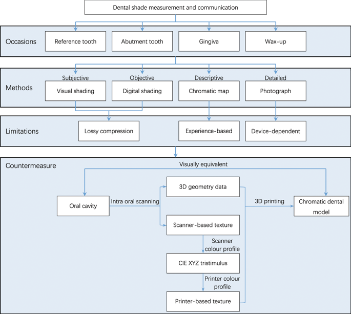
An intra oral scanner (TRIOS 3, 3Shape A/S, Denmark) and a 3D printer (J750, Stratasys Ltd., Israel) were used to build the 3D colour reproduction system. The 3D digital model was captured using the scanner, and saved as a virtual reality modelling language (VRML) file composed of geometry data and texture images. The scanner-based RGB values of each pixel from the texture image were converted to device-independent CIE XYZ tristimulus values using the scanner colour profile, and then to printer-based RGB values using the printer colour profile. The original scanner-based texture images of the VRML model file were replaced with the converted printer-based texture images. Finally, the modified 3D digital model was printed using the 3D printer to produce a physical 3D colour model (Fig. 1).
Development of colour profile for intra oral scanner
A crucial part of this research was the development of the colour profile for the intra oral scanner. This profile would link the RGB values of the scanner’s texture image to device-independent CIE XYZ tristimulus values.
A colour chart (ColorChecker Digital SG, X-Rite Inc., USA) (Fig. 2) provided colour patches. Excluding the outermost greyscale patches, 96 patches were selected from the chart for this process. The spectral reflectance of each patch was measured using a spectrophotometer (ColorEye 7000A, X-Rite Inc., USA). The CIE standard D65 illuminant [I(λ)] and 2° standard observer colour matching functions [(bar{x}(lambda )), (bar{y}(lambda )) and (bar{z}(lambda ))] were selected to calculate CIE XYZ tristimulus values based on the spectral data [S(λ)]:
$$begin{array}{rcl}X & = & frac{100}{N}{int }_{380}^{780},S(lambda )I(lambda )bar{x}(lambda )dlambda ,\ Y & = & frac{100}{N}{int }_{380}^{780},S(lambda )I(lambda )bar{y}(lambda )dlambda ,\ Z & = & frac{100}{N}{int }_{380}^{780},S(lambda )I(lambda )bar{z}(lambda )dlambda ,end{array}$$
where
$$N={int }_{380}^{780},I(lambda )bar{y}(lambda )dlambda .$$
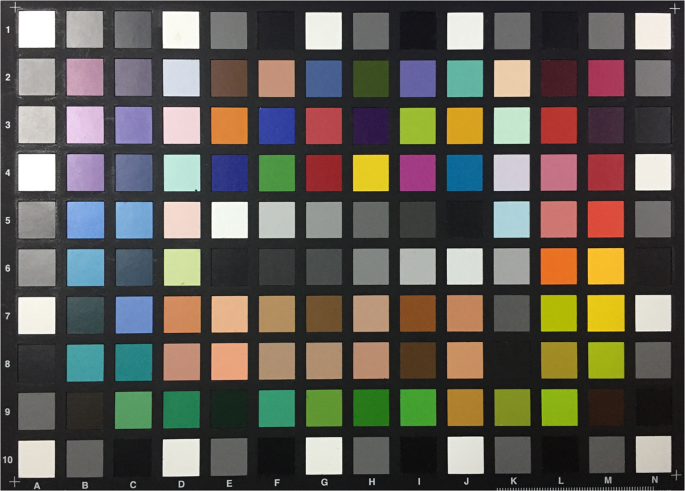
Conventional colour chart used for colour profile development.
The D65 illuminant and 2° standard observer were selected to simulate the practical requirements of dental shading which is generally bright neutral daylight and with a distance of about 1.5 m.
Each patch was then digitized by the intra oral scanner calibrated according to the manual. The “quality” of the colour acquired by the scanner was monitored using the built-in “Shade” function. Any target area marked blue would undergo additional scans from different angles to get correct colour representation (Fig. 3). The digital models were saved as VRML files. The central circular area of each texture image (radius 425 pixels) containing 567,460 pixels (Fig. 4) was selected to calculate average RGB values using Photoshop CC 2014 (Adobe Systems Inc., USA). To normalize the data sets, CIE XYZ tristimulus values were divided by the white point of D65 illuminant (95.047, 100, and 108.883) and the RGB values were divided by 255.
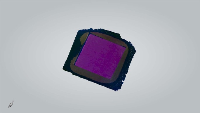
Colour patch digitized by the intra oral scanner.
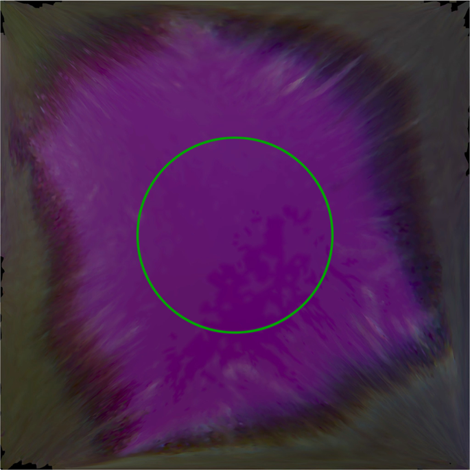
Texture image captured by the intra oral scanner. The green circle marks the area selected for RGB measurement.
The colour profile represents a mathematical model calculated to relate the original RGB values and the target CIE XYZ tristimulus values. Conventional polynomial regression based on least squares is chosen for its convenient implementation and accurate results9,10,11. In this case, the mathematical relationship can be represented as
where T denotes an n × 3 matrix composed of the normalized CIE XYZ tristimulus values of the target colour patch, O denotes an n × p matrix composed of the normalized RGB values and their polynomial terms of the texture image (where n is the number of colour patches and p is the number of terms in the polynomial), and M is the transfer matrix we seek. Therefore, the least-square solution of M is
$$M={({O}^{T}O)}^{-1}{O}^{T}T.$$
For simple linear regression, each row of O represents the normalized RGB values and a constant (usually 1) of a colour patch. The number of terms p therefore is 4, and
$$O=[begin{array}{cccc}1 & {R}_{1} & {G}_{1} & {B}_{1}\ vdots & vdots & vdots & vdots \ 1 & {R}_{n} & {G}_{n} & {B}_{n}end{array}].$$
However, simple linear regression often cannot produce results with acceptable accuracy, thus quadratic and cubic polynomial regressions with more terms are considered. For the quadratic polynomial regression, p is 10, and
$$O=[begin{array}{cccccccccc}1 & {{rm{R}}}_{1} & {{rm{G}}}_{1} & {B}_{1} & {R}_{1}^{2} & {G}_{1}^{2} & {B}_{1}^{2} & {{rm{R}}}_{1}{{rm{G}}}_{1} & {{rm{R}}}_{1}{B}_{1} & {{rm{G}}}_{1}{B}_{1}\ vdots & vdots & vdots & vdots & vdots & vdots & vdots & vdots & vdots & vdots \ 1 & {{rm{R}}}_{n} & {{rm{G}}}_{n} & {B}_{n} & {{rm{R}}}_{{rm{n}}}^{2} & {{rm{G}}}_{{rm{n}}}^{2} & {{rm{B}}}_{{rm{n}}}^{2} & {{rm{R}}}_{n}{{rm{G}}}_{n} & {{rm{R}}}_{n}{B}_{n} & {{rm{G}}}_{n}{B}_{n}end{array}].$$
For the cubic polynomial regression, p is 20, and
$$O=[begin{array}{cccccccccccccccccccc}1 & {{rm{R}}}_{1} & {{rm{G}}}_{1} & {{rm{B}}}_{1} & {{rm{R}}}_{1}^{2} & {{rm{G}}}_{1}^{2} & {{rm{B}}}_{1}^{2} & {{rm{R}}}_{1}{{rm{G}}}_{1} & {{rm{R}}}_{1}{{rm{B}}}_{1} & {{rm{G}}}_{1}{{rm{B}}}_{1} & {{rm{R}}}_{1}^{3} & {{rm{G}}}_{1}^{3} & {{rm{B}}}_{1}^{3} & {{rm{R}}}_{1}^{2}{{rm{G}}}_{1} & {{rm{R}}}_{1}^{2}{{rm{B}}}_{1} & {{rm{G}}}_{1}^{2}{{rm{R}}}_{1} & {{rm{G}}}_{1}^{2}{{rm{B}}}_{1} & {{rm{B}}}_{1}^{2}{{rm{R}}}_{1} & {{rm{B}}}_{1}^{2}{{rm{G}}}_{1} & {{rm{R}}}_{1}{{rm{G}}}_{1}{{rm{B}}}_{1}\ vdots & vdots & vdots & vdots & vdots & vdots & vdots & vdots & vdots & vdots & vdots & vdots & vdots & vdots & vdots & vdots & vdots & vdots & vdots & vdots \ 1 & {{rm{R}}}_{n} & {{rm{G}}}_{n} & {B}_{n} & {{rm{R}}}_{{rm{n}}}^{2} & {{rm{G}}}_{{rm{n}}}^{2} & {{rm{B}}}_{{rm{n}}}^{2} & {{rm{R}}}_{n}{{rm{G}}}_{n} & {{rm{R}}}_{n}{B}_{n} & {{rm{G}}}_{n}{B}_{n} & {{rm{R}}}_{{rm{n}}}^{3} & {{rm{G}}}_{{rm{n}}}^{3} & {{rm{B}}}_{{rm{n}}}^{3} & {{rm{R}}}_{{rm{n}}}^{2}{{rm{G}}}_{{rm{n}}} & {{rm{R}}}_{{rm{n}}}^{2}{{rm{B}}}_{{rm{n}}} & {{rm{G}}}_{{rm{n}}}^{2}{{rm{R}}}_{{rm{n}}} & {{rm{G}}}_{{rm{n}}}^{2}{{rm{B}}}_{{rm{n}}} & {{rm{B}}}_{{rm{n}}}^{2}{{rm{R}}}_{{rm{n}}} & {{rm{B}}}_{{rm{n}}}^{2}{{rm{G}}}_{{rm{n}}} & {{rm{R}}}_{{rm{n}}}{{rm{G}}}_{{rm{n}}}{{rm{B}}}_{{rm{n}}}end{array}].$$
In theory, there is no limitation on the order and number of terms in the polynomial. However, considering the number of samples available, the cost of computing and the required accuracy, the polynomial was constrained. Previous works9,10,11,12,13 indicate that quadratic and cubic polynomials might be suitable here. Adjusted R-squares were adopted for both models to evaluate their accuracy. All the calculations were performed via programming using the C++/Qt5 and C++/Eigen3 libraries.
Development of colour profile for 3D printer
Another crucial part of this research was the development of colour profile for the 3D printer. Different from the scanner colour profile, the printer profile would convert the device-independent CIE XYZ tristimulus values to printer-based RGB values.
The digital models of the colour patches were cropped and reconstructed to blocks of 13 mm (length) * 13 mm (width) * 4 mm (height), and were aligned together to form a 3D colour chart (Fig. 5). The colour chart was printed by the 3D printer using its “High Quality” and matte surface finishing mode (Fig. 6). The spectral reflectance of each block of the 3D colour chart was also measured using the spectrophotometer and was calculated to CIE XYZ tristimulus values under the same condition. The relationship between these CIE XYZ tristimulus values of the printed blocks and their corresponding RGB values was also resolved using polynomial regression based on least squares, as described above, in which the target matrix T was composed of the normalized RGB values of the texture images and the original matrix O was composed of the normalized CIE XYZ tristimulus values and their polynomial terms for the printed blocks. Both quadratic and cubic polynomials were resolved. Adjusted R-squares were adopted for both models to evaluate their accuracy.
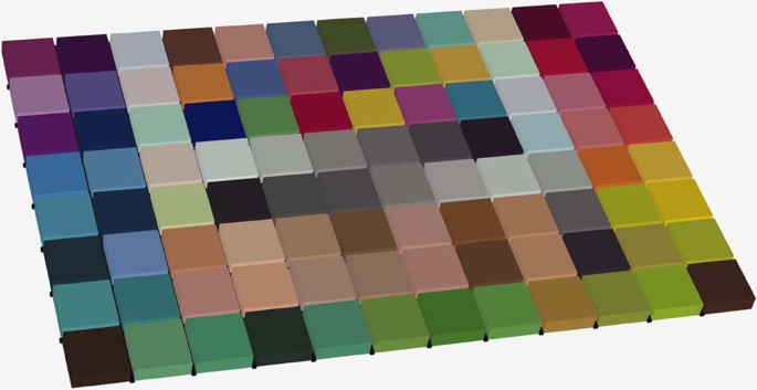
Reconstructed 3D colour chart.
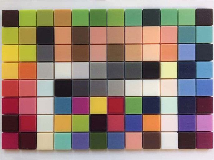
Directly printed 3D colour chart.
Preliminary evaluation of the 3D colour reproduction system
As the CIE XYZ colour space is not particularly perceptually uniform, in order to evaluate the reproduction accuracy in terms of human visual perception, the CIE XYZ tristimulus values of the original colour chart and the printed colour chart are transformed to the CIE L*a*b* colour space according to the following formulas:
$$begin{array}{rcl}{L}^{ast } & = & 116f(frac{Y}{{Y}_{n}})-16,\ {a}^{ast } & = & 500(f(frac{X}{{X}_{n}})-f(frac{Y}{{Y}_{n}})),\ {b}^{ast } & = & 200(f(frac{Y}{{Y}_{n}})-f(frac{Z}{{Z}_{n}})),end{array}$$
where
$$begin{array}{rcl}f(t) & = & {begin{array}{cc}sqrt[3]{t}, & t > {delta }^{3},\ frac{t}{3{delta }^{2}}+frac{4}{29}, & {rm{otherwise}},end{array}\ delta & = & frac{6}{29}.end{array}$$
For D65 illuminant white point, Xn = 95.047, Yn = 100 and Zn = 108.883.
The difference of colours between the corresponding patches from the original 2D colour chart and the directly printed 3D colour charts can be calculated:
$$Delta {E}_{ab}^{ast }=sqrt{Delta {L}^{ast 2}+Delta {a}^{ast 2}+Delta {b}^{ast 2}}.$$
where (Delta {L}^{ast }), (Delta {a}^{ast }) and (Delta {b}^{ast }) respectively represent the differences of the two colours in the L*, a*, and b* parameters.
Given the compatibility of the profiles of the scanner and the printer, different profile combination might result in different colour reproduction performance. In order to select the most suitable combination of profiles, the texture images of the 3D colour chart were adjusted using four profile combinations: quadratic scanner profile – quadratic printer profile (QS-QP), quadratic scanner profile – cubic printer profile (QS-CP), cubic scanner profile – quadratic printer profile (CS-QP) and cubic scanner profile – cubic printer profile (CS-CP). The four adjusted 3D colour charts were printed using the configuration described above. The colour difference of each patch in the 3D colour charts was also measured and calculated. The combination with the lowest overall colour difference (CS-CP) was chosen for in vitro evaluation of tooth and gum shades.
In vitro evaluation of tooth and gum shades of the 3D colour reproduction system
After different colour profiles were created and evaluated, the CS-CP profile combination was chosen to test on tooth and gum shades for the assessment of dental applications. The intraoral scanner digitized 18 resin blocks, including 16 body shades (A1 to D4) and two gum shades (GUM-L and GUM-D) (Ceramage, Shofu Inc., Japan). The digital models were reconstructed, and the textures were adjusted according to the workflow in Fig. 1. The reconstructed and adjusted models were printed by the 3D printer. The CIE L*a*b* values of the original resin blocks and the printed samples were calculated as described above. Calculation of the corresponding (Delta {E}_{ab}^{ast }) evaluated the accuracy of this 3D colour reproduction system.
Statistical analysis
To evaluate the difference of (Delta {E}_{ab}^{ast }) for each profile combination, the non-parametric Friedman test was used following the Shapiro–Wilk test of normal distribution. The null hypothesis was that (Delta {E}_{ab}^{ast }) for each profile combination presented no difference. The results of in vitro evaluation for tooth and gum shades were simply analysed using the mean and median considering the small sample size.


