The study protocol was approved by the Institutional Review Board (IRB) of our institutes (Tokyo Dental College, No. 1091, 2021-12-17). All methods were carried out in accordance with the Helsinki Declaration principles and relevant guidelines and regulations. Informed consent was obtained from all the patients, and written informed consent was obtained from three patients, including the facial images, allowing us to use their information/images in an online open-access publication.
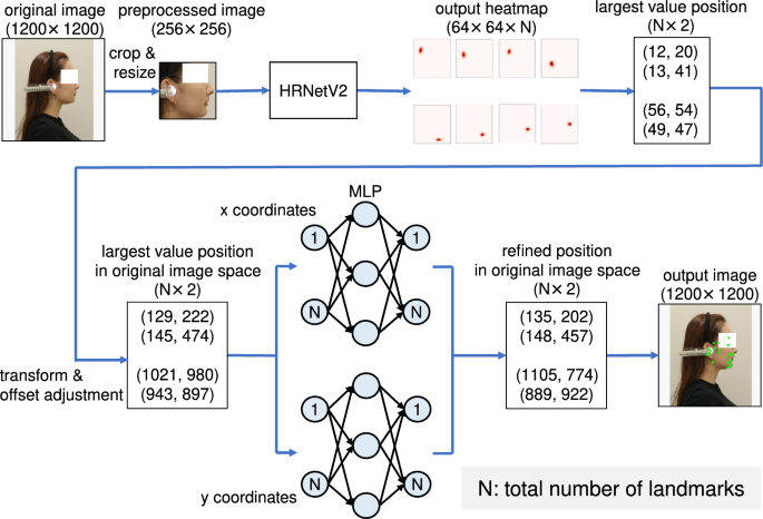
Figure 1 presents an overview of the proposed method. The proposed method comprises two stages: HRNetV231 and MLP. Unlike with existing studies, we used the facial profile images as input instead of a cephalogram. First, all landmark locations in the input images are estimated through heatmap regression using HRNetV2. In this step, the model learns the relationship between the local features of the image and landmarks. As described later in Ablation Study section, the accuracy of the estimation is insufficient, however. Therefore, we introduced a coordinate regression by MLP, which significantly improved the accuracy of landmark estimation. MLP was adopted to estimate the spatial location of the landmarks, i.e., their relative location. This two-stage approach, coarse estimation using heatmap regression and a fine estimation using MLP, enables the accurate detection of all landmarks.

Overview of the proposed model. The model is divided into HRNetV2 and MLP. After HRNetV2 applies the heatmap regression based on the feature extraction, MLP estimates the coordinates based on the spatial relationship of the landmarks.

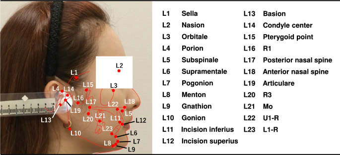
Illustration of 23 cephalometric landmarks.

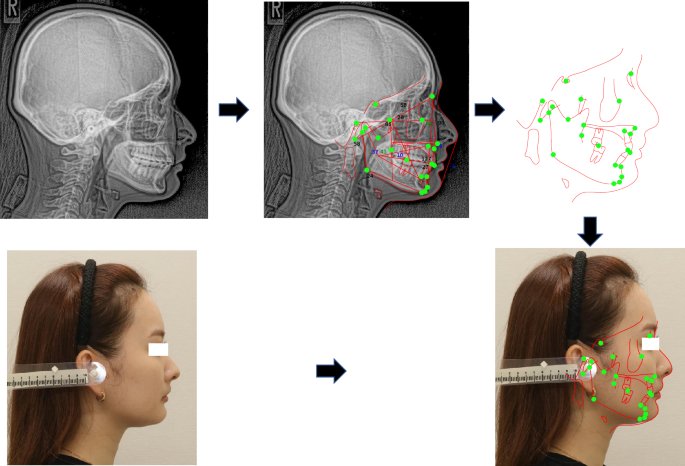
Procedure for plotting landmarks and superimposing the cephalometric tracing on the facial profile image.

HRNetV2 structure31. HRNetV2 comprises four stages connected in parallel by high- to low-resolution subnetworks. The horizontal and vertical sizes of the feature maps correspond to the resolution and number of channels, respectively.

Illustration of how to aggregate information of multiple resolutions using an exchange unit32. A stride (3times 3) convolution is adopted for downsampling. Nearest neighbor sampling followed by a (1times 1) convolution is used for upsampling.
Dataset
A total of 2000 lateral cephalograms and profile photograph images collected from 2000 female patients aged 14 to 69 years (mean age of 27 years) were provided by the Tokyo Dental College. These images were acquired in jpeg format using a CX-150S (ASAHIROENTGEN, Tokyo, Japan) and an EOS Kiss X90 (Canon, Tokyo, Japan). The standard for taking lateral cephalogram is set worldwide. The film should be kept parallel to the mid-sagittal plane of the head and set the head with ear rods so that the center line of the X-ray beam passes through the axes of the left and right ear rods. The distances from the X-ray tube to the mid-sagittal plane of the head and from the mid-sagittal plane of the head to the film is assumed to be 150 cm and 15 cm, respectively. The method of taking a profile photograph image is the same as that of a lateral cephalogram. That is, the distance from the camera to the midsagittal plane of the head is 150 cm, and the head is fixed with ear rods. The skeletal information obtained from the lateral cephalograms was superimposed on the profile photograph images using Quick Ceph Studio (ver. 5.0.2, Quick Ceph Systems, San Diego, California). The 23 landmarks illustrated in Fig. 2 were manually plotted by two orthodontists and finally checked by an experienced orthodontist. The two of them are the board members of Orthodontic specialists. These 23 landmarks were selected from the measurement points of the Downs method, Northwestern method, and a Ricketts analysis. Coordinates of landmarks on the lateral image were identified by imglab, an annotation tool included with Dlib35. Each image has (1200times 1200) pixels and the pixel spacing for the device was 0.35. We present the averaged results of the experiment based on fivefold cross-validation, each containing 400 test and 1600 training profile photograph images, respectively.
Superimposition of the cephalometric tracing on the facial profile image
Figure 3 shows the procedure for plotting landmarks and superimposing the cephalometric tracing on the facial profile image conducted as follows:
- 1.
Plot 23 landmarks and trace the profile (from forehead to upper lip) on the cephalogram within the computer screen of Orthodontic analysis software (Quick Ceph Studio).
- 2.
Separate the set of the landmark plots and the cephalometric tracing on the screen.
- 3.
Superimpose the cephalometric tracing on the facial profile image by manually matching the line from nose to upper lip of the tracing with that of the facial profile image on another screen.
Five sets of the landmark plots and the cephalometric tracing created in step 1 were randomly selected and the same set was superimposed on the facial profile image by each observer according to steps 2 and 3. We measured the intra- and inter-observer landmark distance errors for five landmarks (Sella, Porion, Menton, Gonion, Basion) to confirm the accuracy and reliability of the superimposition. The reason of selecting the five landmarks, it can be considered that the further away from the profile tracing line the larger the error because the superimposition is conducted based on the profile tracing line as shown in step 3. Therefore, the five points farthest from the profile tracing line were selected. To evaluate intra-observer variability, superimpositions were conducted by one orthodontist three times with an interval of two weeks. To evaluate inter-observer variability, superimpositions were conducted by three orthodontists. The two of them are the board member of Orthodontic specialist. The mean and standard deviation of the intra- and inter-observer landmark distance error and the intraclass correlation coefficient (ICC) for the landmark plots were calculated for each set with 95% confidence intervals. In calculating the ICC, the Shapiro-Wilk test was used to determine whether the data were normally distributed. All statistical evaluations were conducted by SPSS software (ver. 27.0, IBM, Armok, New York).
Repeatability and reproducibility test of manual landmark plotting
To compare the repeatability and reproducibility of orthodontists’ landmark prediction errors, a total of five cephalograms from five patients were randomly selected and 23 landmarks were plotted. To evaluate intra-observer variability, cephalometric landmark plotting was conducted by one orthodontist three times with an interval of two weeks. To evaluate inter-observer variability, cephalometric landmark plotting was conducted by three orthodontists. The mean and standard deviation of the intra- and inter-observer prediction error and the ICC for each landmark were calculated for each set with 95% confidence intervals. In calculating the ICC, the Shapiro-Wilk test was used to determine whether the data were normally distributed. All statistical evaluations were conducted by SPSS software.
Heatmap regression
To estimate the location of landmarks, we used HRNetV2 to generate heatmaps of the landmarks. Figure 4 shows the structure of HRNetV231, which starts with a high-resolution subnetwork (stem) and adds high- to low-resolution subnetworks successively to form a stage. The multi-resolution subnetworks are connected in parallel to form a total of four stages. The second, third, and fourth stages are set up by repeating the modularized multi-resolution blocks. The exchange unit, as illustrated in Fig. 5, aggregates the information of each resolution from other subnetworks32. Strided (3times 3) convolutions with stride 2 and a simple nearest neighbor sampling are applied for downsampling and upsampling, respectively. The last exchange unit outputs a feature map where the low-resolution representation is upsampled and concatenated into a high-resolution representation. The heatmap is regressed from the high-resolution representation. A previous study31 reported that the performance is enhanced by employing all resolution representations in comparison to solely using a high-resolution representation.
The ground truth heatmaps are defined as 2D gaussian functions with standard deviation of (sigma) centered on the ground truth location of (textbf{L}_i^G):
$$begin{aligned} h_i^G (textbf{x};sigma ) = frac{1}{2pi sigma ^2}exp {biggl (-frac{Vert textbf{x} – textbf{L}_i^GVert _2^2}{2sigma ^2}biggl )}, end{aligned}$$
(1)
where, (textbf{x}), (i={1,… N}), and (N(=23)) represent the heatmap pixel, index of the landmarks, and total number of landmarks, respectively. To converge the estimated landmarks as close as possible to the ground truth landmarks, the loss function employs the (L_{2}) loss as follows:
$$begin{aligned} L_c = sum _{k=1}^N Vert h_i^G (textbf{x};sigma ) – h_i^P (textbf{x};textbf{w})Vert _2^2, end{aligned}$$
(2)
where (h_i^P (textbf{x};textbf{w})) represents the estimated heatmap, and (textbf{w}) denotes the weights and biases of the network. The loss function allows the network to learn the relationship between the local features and landmarks. The heatmap comprises a 2D matrix with 23 channels corresponding to the number of landmarks. The estimated coordinates (textbf{L}_i^P) of each landmark are predicted by transforming from the reduced space to the original image space. We adjusted the offset of the largest value position from the largest value to the second largest value36. Accordingly, the estimated position can be expressed as a set of 2D coordinates ({textbf{x}^P_i, textbf{y}^P_i}_{i=1}^N).
Coordinate regression
MLP is a refinement of coordinates estimated using spatial relationships between landmarks. It has a simple three-layer structure with an input layer, a hidden layer, and an output layer. Because this is a simple regression task, we adopted a simple MLP to reduce the possibility of an overfitting. In2, a linear filter was also employed to refine the landmark positions; however, only some landmarks were adjusted, and the inputs were the combination of outputs from the two models when considering spatial information. The estimated coordinates ({textbf{x}^P_i, textbf{y}^P_i}_{i=1}^N) are divided into ({textbf{x}^P_1,…,textbf{x}^P_N}) and ({textbf{y}^P_1,… ,textbf{y}^P_N}). The x– and y-coordinates are input into separate models. We adopted the (L_{2}) loss as the loss function to get closer to the ground truth landmarks by using the positional relationship of the landmarks:
$$begin{aligned} L^x_n&= sum _{k=1}^N Vert textbf{x}^G_i – textbf{x}^R_iVert _2^2, end{aligned}$$
(3)
$$begin{aligned} L^x_n&= sum _{k=1}^N Vert textbf{y}^G_i – textbf{y}^R_iVert _2^2, end{aligned}$$
(4)
where (textbf{x}^G_i) and (textbf{y}^G_i) represent the ground truth coordinates, and (textbf{x}^R_i) and (textbf{y}^R_i) denote the refined coordinates. Losses in the MLP were not propagated to HRNetV2, and were learned independently. The number of training epochs for HRNetV2 and MLP differed. For each epoch used for training HRNetV2, we trained the MLP with multiple epochs, provided that we initialized the parameters only at the beginning of training. This procedure allowed us to train the entire model efficiently, while fine-tuning the MLP to match the training phase of HRNetV2.
Implementation details
We trained and carried out testing using a GeForce GTX 1080, 3.70-GHz Intel(R) Core(TM) i7-8700K CPU, and 16GB of memory. The training and testing were conducted in Pytorch. The input images were cropped and resized to (256times 256), according to the center positions of the boxes.
The HRNetV2 network starts with a stem comprising two strided (3times 3) convolutions, which reduces the resolution to 1/4. As the inputs pass through the four subsequent stages, the resolution is gradually reduced by half, and the number of channels is accordingly doubled. The first stage contains four residual units, each of which was formed by a bottleneck with a width of 64. This stage is followed by a (3times 3) convolution, which reduces the width of the feature map to 18. Thus, the number of channels for the four resolutions is 18, 36, 72, and 144, respectively. The second, third, and fourth stages contain one, four, and three multi-resolution blocks, respectively. One multi-resolution block contains four residual units. Each unit contains two (3times 3) convolutions for each resolution and an exchange unit across resolutions. The four resolution representations from the fourth stage are concatenated and used to predict heatmaps with a width of 64, following two (1times 1) convolutions. We trained HRNetV2 with 60 epochs and a batch size of 16. The model was pre-trained using WFLW37. The base learning rate was set as 0.0001, and then was reduced to 0.00001 and 0.000001 at 30 and 50 epochs, respectively. The loss function was minimized using the Adam optimizer.
The MLP network comprises three layers: input, hidden, and output layers. The number of neurons in the middle layer was set to 500. The number of inputs and outputs was set to 23 for splitting the coordinates transformed from the heatmaps and predicted by HRNetV2 into x– and y-coordinates. We trained the MLP using 100 epochs and a batch size of 16 every time HRNetV2 was trained for 1 epoch. The loss function was minimized using the Adam optimizer with a learning rate of 0.00001 and a weight decay (L2 regularization) factor of 0.0001.
Evaluation metrics
We evaluated the proposed method in terms of the mean radial error (MRE), successful detection rate (SDR), and successful classification rate (SCR), according to a previous benchmark study13. The radius error was defined by (R=sqrt{varDelta x^2+varDelta y^2}), where (varDelta x) and (varDelta y) represent the Euclidean distances between the estimated landmarks and the ground truth landmarks of the x– and y-axes, respectively. The MRE and the standard deviation (SD) are defined as follows:
$$begin{aligned} textrm{MRE}&= frac{sum _{i=1}^N R_i}{n}, end{aligned}$$
(5)
$$begin{aligned} textrm{SD}&= sqrt{frac{sum _{i=1}^N (R_i-MRE)^2}{n-1}}, end{aligned}$$
(6)
where (R_i) represents the radial error of the ith landmark, and n denotes the total number of landmarks to be detected. The SDR is the ratio of estimated landmarks that are within a reference threshold, and is defined as follows:
$$begin{aligned} SDR = frac{n_d}{n}times 100%, end{aligned}$$
(7)
where (n_d) represents the number of successfully detected landmarks, and the threshold values are 2.0, 2.5, 3.0, and 4.0 mm, as typically used. The SCR is the classification accuracy of anatomical face types based on eight clinical measures (ANB, SNB, SNA, overbite depth indicator (ODI), anteroposterior dysplasia indicator (APDI), facial height index (FHI), frankfurt mandibular angle (FMA), modified wits (MW)). Facial images are classified into three anatomical types under clinical measures. Note that geometric criteria such as the angles and distances between landmarks listed in Table 1 are considered.

