Comparison of deep learning segmentation and multigrader-annotated mandibular canals of multicenter CBCT scans

Data collection and cohort description

The CBCT imaging data was acquired from the Cranio and Dentomaxillofacial Radiological Department of the University Hospital of Tampere (TAUH), Finland as the first cohort, and from the Department of Oral Radiology, Faculty of Dentistry, Chiang Mai University (CMU), Thailand as the second cohort. All the data in this study is from a normal clinical workflow that represents pre- and postoperative examinations of patients of 10 to 95 years old. The reasons for radiological examination include normal findings and anatomy, but also various traumas, benign or malign pathological conditions, and syndromes. The CBCT scans were randomly and retrospectively selected and pseudonymised, before the annotation process.

The collected dataset of CBCT scans consisted of 1103 individuals, with 869 Finnish patients (79%) and 234 Thai patients (21%). In the Finnish population, with the mean age of 53.7 years, 56% were females and 44% males. The Thai patient population with the mean age of 39.8 years, consisted of 51% females and 49% males. In the dataset, 649 CBCT scans (57%) were imaged using ProMax 3D Max/Mid; (Planmeca, Helsinki, Finland), 125 (11%) using Viso G7; (Planmeca, Helsinki, Finland), 124 (11%) using Scanora 3Dx; (Soredex, Tuusula, Finland), 120 (11%) using DentiScan; (The National Science and Technology Development Agency, Pathum Thani, Thailand), and 114 (10%) using GiANO HR; (NewTom, Bologna, Italy). The first three scanners were used in the first cohort and the latter two scanners in the second cohort. The scan resolution ranged from 0.1 to 0.6 mm isotropic voxel-sizes with most commonly 0.2 mm (59%), 0.4 mm (23%) or 0.3 mm (13%). All the volumes were resampled into 0.4 mm isotropic voxel spacing using linear interpolation before deep learning analysis. Human annotators had access to the scans in the original resolution and could augment the view of the scans using software tools.

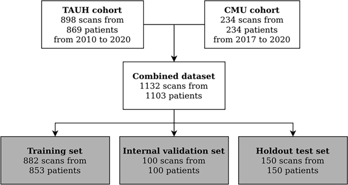
The deep learning methodology is driven by data such that in order to estimate the performance of the model, a partition of the data is held out and only used for validation of the results. This set is called the test set and it was randomly selected with uniform distribution of scanners. The rest of the data was used for the DLS development, and thus called the development set. Flowchart for data collection is presented in Fig. 1.

Flowchart for data collection. Patients were selected from recent clinical workflows at the Cranio and Dentomaxillofacial Radiological Department of the University Hospital of Tampere, Finland (TAUH), and from the Department of Oral Radiology, Faculty of Dentistry, Chiang Mai University (CMU), Thailand. Combined dataset had a total number of 1132 scans from 1103 patients that were split into a training set, internal validation set, and holdout test set with 853, 100, and 150 patients, respectively.

The mandibular canal was annotated using Planmeca developed Romexis 4.6.2. software, which has a built-in tool for mandibular canal annotation using control points and spline interpolation. The control points were standardised to be 3 mm apart from each other, and in the foramen mentale curvature area the canal was annotated using multiple control points, when necessary. Four dentomaxillofacial radiologists participated in this study referred to as Expert 1–4. Experts 1, 3, and 4 are working as senior specialists in TAUH, having 11–35 years of experience in dentistry and Expert 2 who works as a senior consultant in the private sector with 35 years of experience in dentistry. The annotation of the development set was performed by Experts 3 and 4 with 90% and 10% proportions of the set, respectively. The test set was annotated independently by all radiologists. Since the end-point of the mandibular canal in the mandibular foramen region is ambiguous, the end-point was selected to match the shortest annotation in the superior direction, thus improving the sensitivity of the canal localization in the foramen mentale and dental regions rather than highlighting differences in the canal path lengths. The set was also subjectively annotated for the clarity of mandibular canal visibility to be either Clear or Unclear. The test set scans were also annotated for the following conditions if present: movement artefact, bisagittal osteotomy, metal artefact, difficult pathology, and difficult bone structure including difficult anatomy and osteoporosis.

This study is based on a retrospective and registration dataset and as such does not involve experiments on humans and/or the use of human tissue samples and no patients were imaged for this study. A registration and retrospective study does not need ethical permission or informed consent from subjects according to the law of Finland (Medical Research Act (488/1999) and Act on Secondary Use of Health and Social Data (552/2019)) and according to European General Data Protection Regulation (GDPR) rules 216/679. The use of the Finnish imaging data was accepted by the Tampere University Hospital Research Director, Finland October 1, 2019 (vote number R20558). Certificate of Ethical Clearance for the Thai imaging data was given by the Human Experimentation Committee, Faculty of Dentistry, Chiang Mai University, Thailand (vote number 33/2021) July 5, 2021. According to the Thailand legislation informed consent was not needed.

Validation of the deep learning system

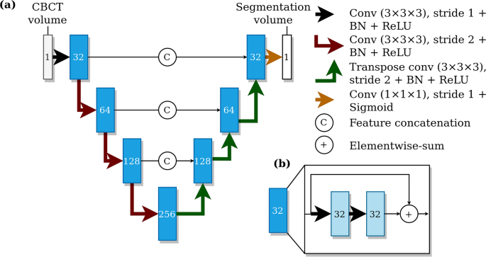
We utilised the previously proposed CNN-based method⁴ as our deep learning model, i.e. a type of fully convolutional neural network using a U-net style architecture¹². The model utilises three dimensional convolutional layers that enables the recognition of patterns in axial, coronal, and sagittal planes, simultaneously. The model was trained with volume patches from randomly flipped and translated volumes using the Dice-loss objective for 60 epochs. The model parameters were updated using the Adam optimizer¹³ and the final parameters were selected from checkpoints after each training epoch, based on the best validation set performance. The model architecture is shown in Fig. 2. We developed an improvement to the canal extraction post processing algorithm from the model segmentation. In short, mandibular canal route segments are obtained from the CNN output using a skeletonization routine¹⁴, route segments are concatenated using a heuristic, and then the routes with anatomical characteristics of mandibular canals are selected. Finally, the pair of routes with the most symmetricity is chosen as the pair of canals.

The architecture of the deep learning system. (a) A U-net style deep learning system architecture with a contracting pathway and an expanding pathway. The contracting pathway is visualised with red arrows, each marking a convolution block with a stride of two. The expanding pathway is visualised with green arrows, each marking a transpose convolution block with a stride of two. The pathways are connected with feature concatenation marked using arrows with the letter C. The number of feature maps is shown on each block and all the convolutions except the last one have a kernel size of 3 × 3 × 3. The last convolution has one feature, a kernel size of 1 × 1 × 1, no layer normalisation, and uses the sigmoid nonlinearity. (b) Each block includes two convolutions with a stride of one, batch normalisation (BN), and ReLU non-linearities with elementwise summation marked using arrows with a plus sign.

Statistical analysis

For the evaluation of the mandibular canal localization performance, we used the mean curve distance (MCD), similar to previous works^4,7,8, and in addition we propose the symmetric mean curve distance (SMCD). In the case of MCD, for each point, i.e. a three dimensional coordinate, on a ground truth curve, the distance to the closest point on another estimator curve is computed and then these distances are averaged. Thus, it estimates the average distance from one curve to another in three dimensional space. However, by definition, the MCD is computed from the point of view of the ground truth curve, effectively measuring the sensitivity in curve localization, and thus, there are cases when the MCD does not reflect the errors well. For example, if the ground truth curve and estimator curves are well aligned, but the estimator curve is longer from either or from both ends. Hence, we propose the SMCD measure, which is calculated as the average of the MCD values computed both ways. In addition, the SMCD is useful in summarising the interobserver variability, as the role of the ground truth and estimator curves are not well defined. Note that a visualisation of how the MCD is computed is presented in the Supplementary.

In mathematical terms, let T and E be the sets of points that define the ground truth curve and the estimator curve, respectively. We perform the mandibular canal segmentation in three dimensional space, and thus the points are the three dimensional coordinates of the discretized mandibular canal path curves. The point to curve distance function d(x,S) is defined such that it computes the minimum Euclidean distance from a point x to the set of points S that defines a curve:

Then the MCD is computed as:

The SMCD is computed using Eq. (2) and a permutation of the arguments:

We have also evaluated the proportion of the canal path within a 2 mm radius in order to evaluate the localization accuracy that approximates the 2 mm safety margin above the canal that is used as a guideline for implant planning¹¹. Volumetric segmentation measures, such as the Dice similarity coefficient, were deemed unsuitable for our main results, since the annotation tool in our study was designed to use a fixed diameter for the canal. However, the results measured with the Dice similarity coefficient are reported in the Supplementary Figs. S2–S5.

We evaluated and analysed the variability between the Experts and the deep learning system by comparing the radiologists’ canal annotations and the segmentations produced by the deep learning system in a pairwise manner. In order to estimate the highest level of interobserver variability, for each CBCT scan we selected the pair of Expert annotations with the highest mean curve distance. Similarly, we selected one Expert annotation with the highest mean curve distance with the deep learning system, by treating the Expert annotation as the ground truth curve and the automatic segmentation as the estimator, to estimate the highest variability between the system and an Expert. The generalisation capacity of the previously published system⁴ was evaluated similarly by selecting the Expert annotation with the highest mean curve distance to the segmentation produced by the system.

We estimated the objective performance between the Experts and the deep learning model by constructing a label voting scheme of the expert annotations as the reference ‘ground truth’ using SimpleITK library¹⁵ and evaluated the performance using SMCD. Specifically, voxels are assigned a background or mandibular canal label with maximum votes and undecided voxels are marked as a canal label. After this, the segmentation was skeletonized and the curve was determined with connected component analysis. Statistical significance of all the main results were computed using the two-tailed Wilcoxon signed-rank test with alpha value selected at 0.001 using statannotations Python package¹⁶.

Inclusion/exclusion criteria

There was no exclusion criteria in the diagnostically acceptable patient scans.