In this section, we present a detailed description of the deep learning system and its components, describe the patient data used for the results, and the quantitative and qualitative evaluation measures we use to evaluate reproducibility.
Deep learning model
The deep learning system (DLS) we study was proposed in two recent studies13,16. This model was also used as a basis in the work of publicly available voxel level annotated 3D mandibular canal dataset14. The DLS consists of two algorithms; a deep learning neural network that segments the voxels containing the mandibular canals from 3D CBCT volumes, and a postprocessing algorithm that extracts the two most likely mandibular canal curves from the segmentation volume. For our analysis, we utilise the previously trained model16, which was developed on a heterogeneous, multi-device, and multiethnic dataset of 1082 scans to evaluate its temporal generalisability and reproducibility with a new dataset, focused on challenging clinical heterogeneities.
The deep learning model of DLS is a type of fully convolutional neural network with a U-net style architecture17. The model utilises three dimensional convolutional layers that enable the recognition of patterns simultaneously in the axial, coronal, and sagittal planes. The deep learning model produces approximate segmentations of the mandibular canals, which are then postprocessed using connected component analysis for the purpose of reducing false positives as well as connecting partial segmentations to form a single canal. Segmentation is then reduced into a curve using a skeletonisation routine18, and a heuristic concatenation algorithm is used to select and combine curve segments in order to extract the two mandibular canals based on correct anatomical characteristics and symmetry.
Patient data
The data was collected retrospectively from the Tampere University Hospital (TAUH) in Tampere, Finland. The patients whose data had been previously used in the development, validation, or testing of the DLS were excluded. Every patient has at least two CBCT scans imaged for medical reasons. These reasons include benign lesions follow-up, operation planning and control for orthognathic surgery and temporomandibular joint prosthesis, trauma controls, computer assisted surgery planning, and bone destructive lesions including malignancies. The collected dataset of 165 CBCT scans consisted of 72 patients with a mean age of 45.2±17.0 and a range from 17 to 89 years, having 47% males with a mean age of 43.7±15.8 and a range from 20 to 72 years, and 53% females with a mean age of 46.7±18.3 and a range from 17 to 89 years. Patients’ age information was collected according to age at the last repeated scan. The scans were pseudonymised and categorised into four main subgroups to evaluate the effects of different heterogeneities. In addition, the dataset included immediate postoperative scans that were categorised into a separate heterogeneity subgroup, to examine the effect of the surgical operation before the healing process.
Three scanners with different imaging parameters were used; KAVO OP 3D PRO, VISO G7, and Scanora 3Dx with 7, 66, and 92 scans, respectively. The voxel spacing of the scans ranged from 0.2 mm to 0.5 mm with the most common ones being 0.2 mm, 0.3 mm, and 0.4 mm with 57%, 29%, and 7% of the scans, respectively. The dataset consisted of 107 high resolution (HR), 33 standard resolution (SR), 12 low dose (LD), and 13 ultra-low dose (ULD) scans. The distribution of different devices, voxel spacings, and doses are presented in Supplementary Table S1. All the scans were whole facial imaging, large field-of-view scans, due to the aforementioned diagnostic needs in radiological imaging. There were 39 patients with two CBCT scans, and 33 patients with multiple (three to five) scans in the study material. There were 11 patients who were scanned with the same CBCT device and the same imaging parameters, 16 scanned with the same device but different imaging parameters, and 45 who were scanned with different devices and different imaging parameters. All the scans were taken in TAUH from 2015 to 2020.
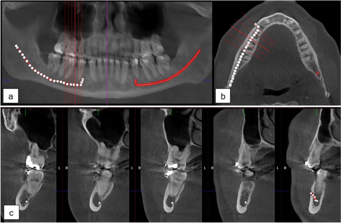
The mandibular canals were annotated using clinical software: Romexis 4.6.2, of Planmeca, Finland, by a senior radiologist with over 35 years of experience in dentistry, similarly to previous works13,16. In the annotation process, a CBCT panoramic reconstruction was made (Fig. 1a), cross-sectional images against panoramic curves were reconstructed (Fig. 1b), and the midline of the canals were marked with standard 1.5 mm diameter control points placed in 3 mm intervals. The whole path of the mandibular canal was marked starting from the foramen mentale opening and ending at the foramen mandibulae opening. Multiple control points were used for each of the canals, especially in the foramen mentale curvature area and in complicated cases (Fig. 1c). An approximate segmentation was created when computing segmentation measures, in which the path of the canal was expanded to a 1.5 mm static diameter tube.
The four main subgroups manifest various clinical and operative situations in dental and maxillofacial radiology, including pre- and postoperative, and follow-up CBCT scans. These subgroups were determined as Normal group, Prosthetic group, Orthognathic surgery group, and Pathological group with 23, 13, 22, 14 patients and 51, 35, 46, 33 scans, respectively.
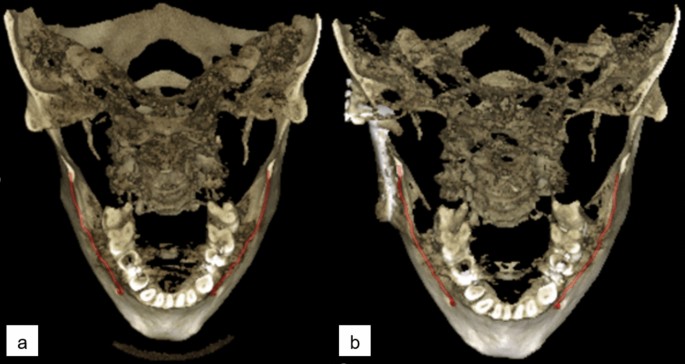
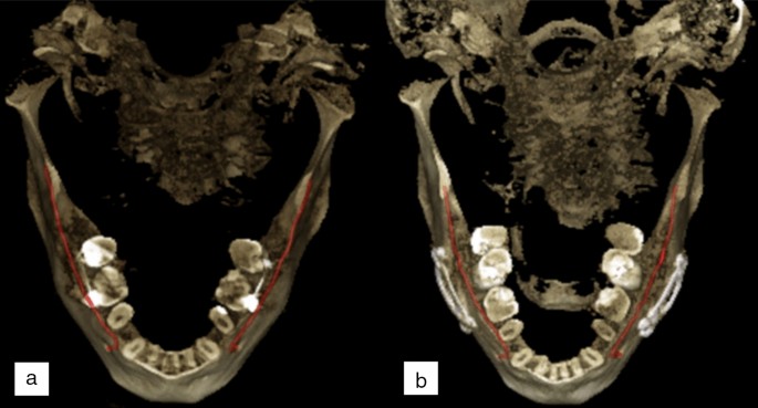
The patients of Normal group were scanned for reasons having no major influence in the mandibular canal area, but 14 of the 51 scans (27%) were reported to have difficult bone structure. The patients of Prosthetic group have major temporomandibular joint (TMJ) disorders and have at least one preoperative scan and one postoperative scan after full prosthetic metallic TMJ-reconstruction. An example of a patient from TMJ Prosthetic group is shown in (Fig. 2). The patients of Orthognathic surgery group have undergone a bilateral sagittal split osteotomy (BSSO), where the mandible is split bilaterally and moved forward or backward, to correct malocclusion and functionality19, and have at least one preoperative and one postoperative scan taken six to 12 months after the operation. The BSSO changes the path of the mandibular canal and fixation materials cause metallic artefacts in the imaged area, both seen as differences between the preoperative scan and postoperative scan of the patient. The effect of this heterogeneity is shown in three dimensional (3D) reconstructions models of preoperative (Fig. 3a) and postoperative (Fig. 3b) cases. The patients of Pathological group have severe pathological bone destructive diseases in the mandible, which may partly or completely destroy the visibility of the mandibular canals, and have at least one preoperative, and one postoperative or follow-up scan. Eight of the 14 patients (57%) had a malignant bone destruction on the right side of the mandible.
The immediate postoperative scans, i.e. those imaged less than five days after the BSSO surgery, were excluded from the main analysis. The visibility of mandibular canal is extremely poor in these scans20 and there are changes to the path of the mandibular canal due to BSSO. Thus, the localisation of the mandibular canal is challenging in these scans. However, the task of localising the mandibular canal in these cases is rarely clinically relevant and thus the analysis is included in the Supplementary.
This study is based on a retrospective and registry-based dataset, and as such does not involve experiments on humans and/or the use of human tissue samples and no patients were imaged for this study. A registration and retrospective study does not need ethical permission or informed consent from subjects according to the law of Finland (Medical Research Act (488/1999) and Act on Secondary Use of Health and Social Data (552/2019)) and according to European General Data Protection Regulation (GDPR) rules 216/679. The use of the data was accepted by the Tampere University Hospital Research Director, Tampere, Finland, 1st of October, 2019 (vote number R20558).

(a) CBCT panoramic reconstruction showing the annotation control points in the left and the interpolated mandibular canal in right side of the mandible, (b) an axial slice with cross-sectional slices along the panoramic curve shown in red, (c) annotation control points in the cross-sectional slices 3 mm apart with multiple annotation points in the foramen mentale area.

Three dimensional reconstruction images with manually annotated mandibular canals shown in red, (a) preoperative CBCT scan, (b) postoperative CBCT scan with right side temporomandibular joint reconstruction on the angulus area of the mandible.

Three dimensional reconstruction images of an orthognathic surgery patient showing changes in the postoperative scan with manually annotated mandibular canals shown in red, (a) preoperative CBCT scan, (b) postoperative CBCT scan 1 year after the operation.
Quantitative analysis approach
In the quantitative analysis, the outputs of the DLS were compared to the senior radiologist’s annotations. The mandibular canal localisation accuracy of the DLS was evaluated using the Symmetric Mean Curve Distance (SMCD)16. In the SMCD, the average deviation between the full path of the radiologist’s annotation and the DLS output is determined. It thus measures how far apart the two curves are on average. In addition, the segmentation performance of the DLS was evaluated using the Dice similarity coefficient (DSC), which is a normalized measure of the intersection of two segmentations, and the average symmetric surface distance (ASSD) that measures the average error between the surfaces of two segmentations. However, these metrics are computed using the senior radiologist’s approximate segmentation of the canal as the ground truth, and thus they only approximate the true segmentation performance.
The reproducibility was evaluated by measuring the temporal variability in SMCD for each canal, i.e. the two canals of each patient were treated as independent subjects of interest. The reproducibility measures we used were the within-subject standard deviation (wSD) and the repeatability coefficient (RC), and we also report the within-subject mean and ranges of values. The wSD estimates the variability in SMCD values for the canals and the RC the largest difference between two SMCD values for the same canal with 95% confidence. These quantities are computed in Eqs. (1) and (2) as follows21:
$$begin{aligned} text {wSD}&= sqrt{text {WMS}}, end{aligned}$$
(1)
$$begin{aligned} text {RC}&= 1.96~sqrt{2}~text {wSD} nonumber \&approx 2.77 text {wSD}, end{aligned}$$
(2)
where WMS is the within-subject mean squared error, computed as:
$$begin{aligned} text {WMS} = sum _{i=1}^n sum _{k=1}^{K_i} frac{(Y_{ik} – {bar{Y}}_i)^2}{n(K-1)}, end{aligned}$$
n is the number subjects, (K_i) the number of repetitions for subject i, (Y_{ik}) the kth measurement of subject i, and ({bar{Y}}_i) the mean of replications of subject i. As our dataset includes variable number of repetitions per subject, the K is computed by applying a downward correction to reduce overestimation of the variation among smaller groups compared to larger groups: (K!=!frac{1}{n-1}left( N-frac{sum _{i=1}^n!K_i^2}{N}right) ), where N is the total number of scans22.
Qualitative analysis approach
For the qualitative analysis, the annotations by the senior radiologist and those produced by the DLS were assessed by three experts; two dental and maxillofacial radiologists with 15 and 13 years of working experience, and one resident of dental and maxillofacial radiology with 8 years of working experience in dentistry.
There were in total 636 mandibular canal segmentations in the comparison: 318 annotated by the radiologist and 318 DLS outputs, which were provided to the three experts independently and in a random order, without informing whether the segmentation was done by the radiologist or by the DLS. In addition, the segmentations were assessed two times by each expert in separate sessions with a two week interval. The observers assessed the quality of each segmentation and its feasibility for clinical diagnostics using a five-point Likert scale defined with 0: not usable for diagnostics, 1: partly usable for diagnostics, canal visibility below one half, 2: minor issues with almost fully usable for diagnostics, 3: almost perfect, fully diagnostically usable, and 4: perfect, fully diagnostically usable. The Likert ratings were also used to form a binary scale for the diagnostic suitability of a canal segmentation. It was defined as Likert ratings 3 and 4 being fully suitable for diagnosis and 0–2 as not fully suitable.
The observers justified their ratings using five pre-selected error types: fully missing, major parts of the segmentation missing, slightly off the centre of the canal, short at the mandibular foramen, and short at the mental foramen. The first and second error types are considered clinically relevant resulting in Likert rating of 0-2 and diagnostically not fully usable. The other three error types have less clinical importance and they can be explained by the anatomy of the mandible, and the nature of the heterogeneity subgroups.
The reproducibility was evaluated using the Likert scores of the first annotation session. Due to the discrete and ordinal nature of the Likert scores, as well as the high consistency of the given scores in the dataset, Gaussian random effects models and analysis of variance methods were deemed unsuitable. In addition, the number of temporal scans varied between the patients, and thus methods that require paired data, such as the Kendall rank correlation coefficient, could not be used to analyse the reproducibility. We utilised a Bayesian statistical analysis approach for the reproducibility of ordinal measurements, proposed in a recent study23. In short, it uses a random effects model, with subject-dependent random effects, combined with the Master’s partial credit model24. It defines the probability that the subject i’s Likert score (y_i) is equal to the number h, given the random effect of the subject (x_i) and grader j specific parameters (alpha _j) and (delta _j), as follows:
$$begin{aligned} p_j(y_i=h mid x_i, alpha _j, delta _j) = frac{exp {(sum _{m=1}^{h-1}alpha _j(x_i-delta _{jm}))}}{sum _{n=1}^Hexp {(sum _{m=1}^{n-1}alpha _j(x_i-delta _{jm}))}}. end{aligned}$$
It should be noted that in computing the probabilities, the Likert scores were mapped from 0–4 to 1–5. A detailed description of the approach is given in the Supplementary material.
We used the repeatability measure (RM) proposed in the aforementioned study to measure the reproducibility. For grader j, it is defined as the probability that two Likert scores for the same segmentation will be the same, averaged over the data in Eq. (3):
$$begin{aligned} {hat{RM}}_j(alpha _j, delta _j) = frac{1}{n} sum _{i=1}^n sum _{h=1}^5 p_j(y_i=h mid x_i, alpha _j, delta _j)^2 end{aligned}$$
(3)
The Bayesian analysis produces a distribution of possible parameter values (alpha _j) and (delta _j), which we used to compute the posterior average (RM_j = Ave_{alpha _j, delta _j}({hat{RM}}_j)) and the 95% credibility intervals for each Expert. The analysis was performed for the full dataset, as well as for each heterogeneity group independently. We implemented the analysis using the Stan25 programming language with the Python interface PyStan26, and using the default settings described in the original study23.
To analyse the intra- and interobserver variability, we calculated the accuracy of Likert ratings. The interobserver variability was evaluated by comparing the assessments between each pair of experts, and the intraobserver variability by comparing the ratings of the first and second assessment session.

