Deep Learning Method for Mandibular Canal Segmentation in Dental Cone Beam Computed Tomography Volumes

Data

The CBCT dataset consisted of 637 scans from 594 patients. The scans were reconstructed from dentomaxillofacial area CBCT scans ranging from partial scans to whole head scans. The scanning devices were Soredex Scanora 3Dx, (Soredex Oy, Tuusula, Finland) and Planmeca ProMax 3D, ProMax 3D Max, ProMax 3D Mid, (Planmeca Oy, Helsinki, Finland). All the scans had isotropic spatial resolution, with 492 scans with voxel spacing of 0.2 mm, 141 scans with voxel spacing of 0.4 mm, and one scan each with 0.1 mm, 0.15 mm, 0.3 mm, and 0.6 mm voxel spacings. The size of the volumes ranged from (291times 251times 251) voxels to (825times 825times 825) voxels. The CBCT scans had the grey values in the (approximated) Hounsfield unit scale, ranging from -1000 to 3095, except for a few erroneously reconstructed scans with artefacts. The data was scanned in the Cranio and Dentomaxillofacial Radiology Department of The University Hospital of Tampere, Finland. All the acquired CBCT scans were pseudonymized.

The dataset was divided into a training, validation, and test sets, with 457, 52, and 128 CBCT scans, respectively. The model parameters were trained on the training set, the model architecture and hyperparameters selected using the validation set, and the final trained model was evaluated on the test set. In order to avoid overoptimistic results due to over-fitting, that is, memorising patient specific features, each of these sets had a unique set of patients. Moreover, the patients with multiple scans were not included in the validation and test sets. As the number of the 0.1 mm, 0.15 mm, 0.3 mm, and 0.6 mm voxel spacing volumes was very small, they were included in the training set. The scans with the 0.2 mm and the 0.4 mm voxel spacing were randomly divided in similar proportions to the different sets. In addition, each set was constructed to maintain a similar distribution of the two measurement devices. However, all the scans were rescaled to 0.4 mm voxel spacing as a preprocessing step, described later.

In a number of cases the patients’ CBCT scans were taken during preoperative and postoperative radiological examinations, which introduced abnormalities of facial anatomy in the scans of these patients. The scans of the operated patients can also include foreign, mostly metallic material, such as dental implants and fixation materials, causing artefacts of varying degree. Other heterogeneities in the scans include motion artefacts, as well as rotations and translations of the head.

Each scan in the test set was scrutinised for various types of abnormalities. The total number of canals affected by a certain abnormality included 8 cases of osteoporosis, 3 cases of pathological condition, such as benign or malignant tumour, 4 cases of difficult anatomy, 49 cases of difficult bone structure, 9 cases of post bisagittal osteoma operation, 4 cases of metal artefacts, and 11 cases of movement artefacts. Also, 2 of the scans were from cadavers, amounting to 4 canals. The total number of canals affected by heterogeneities was 72, with some of the canals having multiple abnormalities affecting them. Additional results considering model performance for each of these heterogeneities are shown in the Supplementary Table S2.

The mandibular canals were annotated by two medical professionals. One of them is a dentomaxillofacial radiologist, with 34 years of experience in dentistry, and the other is a resident of dentomaxillofacial radiology, with 10 years of experience in dentistry. These experts annotated the training set and the secondary test data using Romexis® 4.6.2.R software by Planmeca, specifically the built-in tool for mandibular canal annotation. This tool requires the user to specify control points for the canal, and the software interpolates the pathway of the canal based on the control points. The pathway is then expanded to a 3.0 mm diameter tube and finally discretised to provide the ground truth segmentation volumes. This methodology was used in creating the annotations for the training, validation, and test sets. A visualisation of the model segmentation and the annotation is presented in Fig. 3 for a representative scan. Informed consent was obtained from the subject shown in this figure for the publication.

The sparse specification of the control points and the discretisation of the interpolated tube introduced noise to the ground truth annotations. For accurate evaluation, 15 CBCT volumes were selected from the test set and annotated at the voxel level. The selection was based on clear visibility of the mandibular canals, while preserving the distribution of voxel spacings. As such, there was not any canals affected by the abnormalities in the set. Due to the more labour-intensive and time-consuming nature of the voxel-level annotation, these annotations were only made for model evaluation purposes. The software used for the voxel-level annotation was Mimics inPrint 3.0 software (Materialise, Leuven, Belgium). The 15 CBCT scans with voxel-level annotations served as our primary test data. The full test set with coarse annotations was used as the secondary test data.

In order to standardise the data three preprocessing steps were used. First, all the scans were resized to the 0.4 mm voxel spacing using linear interpolation. This procedure reduced significantly the memory footprint of the largest volumes, such as the whole head scans with 0.2 mm voxel spacing. Second, the values outside the valid Hounsfield unit scale were clipped to the valid range of  ([-1000,3095]). Third, the grey values were then normalised to the interval [0, 1].

The segmentation model

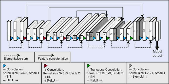
As the backbone of our segmentation method, we used a 3D fully convolutional neural network. A graphical illustration of the model is presented in Fig. 4. The neural network architecture is similar to the U-net¹⁶, and can be divided to a contractive pathway and an expanding pathway. In the contractive pathway, the feature maps are down-sampled with stride 2 convolutions, and in the expanding pathway, the feature maps are up-sampled with stride 2 transpose convolutions. With the exception of the last layer of the neural network, all convolutions and transpose convolutions have the kernel size of (3times 3times 3), and are followed by a batch normalisation operation¹⁹ and a rectified linear unit (ReLU) non-linearity. The last layer of the network has a convolution with the kernel of size (1times 1times 1), and the link function is chosen as the logistic sigmoid. Between the contracting and the expanding pathways are long skip connections, which concatenate the hidden layers along the channel dimension. The network also utilises residual connections²⁰ within each of the down-sampling and up-sampling blocks.

Graphical illustration of our fully convolutional neural network architecture. Each block depicts a hidden layer of the network. The height of each of the blocks visualises the evolution of the spatial size in the network. As a comparison, the depth visualises the evolution of the number of the feature maps in the network. The number of the feature maps of each layer is also shown as a number on each block. The blocks containing concatenation are shown in dark grey. BN and ReLU correspond to the batch normalisation operation and the rectified linear unit non-linearity, respectively.

The CBCT volumes had spatial dimensions that were too large to fit into a workstation graphical processing unit (GPU), using our model. Thus, a patch sampling method was employed, in which (3{2}^{3}) sized patches were randomly sampled using a stride of 22. To reduce the class imbalance, the patches without any mandibular canal voxels were not included in the training set. Each of the sampled patches were augmented with random flips in all the spatial dimensions. The model was trained for 400 epochs using a mini-batch size of 24. Parameter updates were calculated using the Adam algorithm²¹, with the learning rate set to 0.0001, ({beta }_{1}) as 0.9, and ({beta }_{2}) as 0.999.

The network was trained using a differentiable version of the Dice similarity coefficient, which alleviates the class-imbalance problem when calculated for the minority class. The DSC is defined as the intersection of two sets, normalised with the cardinalities of the sets. However, this definition is not differentiable, as it assumes thresholded binary predictions. The Dice loss (DL) used to train our network is based on the soft Dice coefficient objective function, proposed in¹⁷, and is defined as follows, in the Eq. (1):

Here ({t}_{n}) is a binary variable which represents the ground truth label of the voxel indexed by (n), and is 0 for the negative class and 1 for the positive class. ({p}_{n}) is the probability that the voxel indexed by (n) belongs to the positive class, and is determined by the model.

In addition, we developed a post-processing method to refine the model predictions. The raw model output had large quantities of false positives, likely due to sampling the training patches close to the mandibular canal. The output was filtered with a connected-component algorithm that connects neighbouring voxels to larger structures, from which the two largest structures were chosen as the predicted canals. In the model evaluation, the number of canals was known for each volume, and this information was used to select the appropriate number of structures.

Performance measures

In order to measure the performance of the deep learning model, we calculated the DSC, precision, and recall using the following Eqs. (2)–(4):

Here TP denotes the true positives, FP false positives, and FN false negatives.

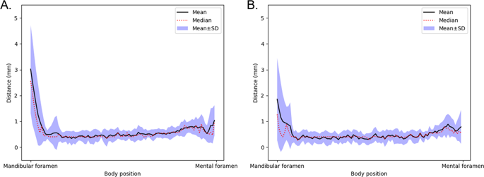
The DSC, precision, and recall give us insight into the voxel-level segmentation performance of the model. However, these measures do not consider the distance from the predictions to the ground truth canal in the patient’s mandible, which is of key importance for example from the dental surgery point of view. In order to include the location based performance measures, we also evaluate the segmentation performance of our model using the following three distance based measures: average symmetric surface distance (ASSD), mean curve distance (MCD) and robust Hausdorff distance (RHD), calculated using the Eqs. (5), (6), and (7), respectively:

Here (d({boldsymbol{b}},B)={min }_{{boldsymbol{b}}in B}left{parallel {boldsymbol{a}}-{boldsymbol{b}}{parallel }_{2}right}). The ({boldsymbol{t}}) denotes the coordinates of a ground truth canal voxel, ({boldsymbol{p}}) the coordinates of a predicted canal voxel, (T) the set of ground truth canal voxel coordinates, (P) the set of predicted canal voxel coordinates, (S(,cdot ,)) an operation which extracts the surface voxels of a set of voxels, (C(,cdot ,)) an operation which extracts the curve line of a set of voxels, in practice implemented as a skeletonization algorithm, and ({P}_{k}) denotes the (k):th percentile.